
diff options
| -rw-r--r-- | .gitignore | 1 | ||||
| -rw-r--r-- | python-gammy.spec | 1320 | ||||
| -rw-r--r-- | sources | 1 |
3 files changed, 1322 insertions, 0 deletions
@@ -0,0 +1 @@ +/gammy-0.5.0.tar.gz diff --git a/python-gammy.spec b/python-gammy.spec new file mode 100644 index 0000000..d0b3212 --- /dev/null +++ b/python-gammy.spec @@ -0,0 +1,1320 @@ +%global _empty_manifest_terminate_build 0 +Name: python-gammy +Version: 0.5.0 +Release: 1 +Summary: Generalized additive models with a Bayesian twist +License: MIT +URL: https://malmgrek.github.io/gammy +Source0: https://mirrors.nju.edu.cn/pypi/web/packages/a2/c5/de836446cc34ef1d8ad8493bf8cad4021b877fae009c4f797b24f748037d/gammy-0.5.0.tar.gz +BuildArch: noarch + +Requires: python3-numpy +Requires: python3-scipy +Requires: python3-bayespy +Requires: python3-h5py +Requires: python3-matplotlib +Requires: python3-ipython +Requires: python3-sphinx +Requires: python3-numpydoc +Requires: python3-pytest + +%description +# Gammy – Generalized additive models in Python with a Bayesian twist + +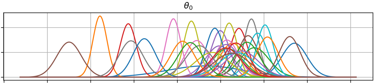 + +A Generalized additive model is a predictive mathematical model defined as a sum +of terms that are calibrated (fitted) with observation data. + +Generalized additive models form a surprisingly general framework for building +models for both production software and scientific research. This Python package +offers tools for building the model terms as decompositions of various basis +functions. It is possible to model the terms e.g. as Gaussian processes (with +reduced dimensionality) of various kernels, as piecewise linear functions, and +as B-splines, among others. Of course, very simple terms like lines and +constants are also supported (these are just very simple basis functions). + +The uncertainty in the weight parameter distributions is modeled using Bayesian +statistical analysis with the help of the superb package +[BayesPy](http://www.bayespy.org/index.html). Alternatively, it is possible to +fit models using just NumPy. + +<!-- markdown-toc start - Don't edit this section. Run M-x markdown-toc-refresh-toc --> +**Table of Contents** + +- [Installation](#installation) +- [Examples](#examples) + - [Polynomial regression on 'roids](#polynomial-regression-on-roids) + - [Predicting with model](#predicting-with-model) + - [Plotting results](#plotting-results) + - [Saving model on hard disk](#saving-model-on-hard-disk) + - [Gaussian process regression](#gaussian-process-regression) + - [More covariance kernels](#more-covariance-kernels) + - [Defining custom kernels](#defining-custom-kernels) + - [Spline regression](#spline-regression) + - [Non-linear manifold regression](#non-linear-manifold-regression) +- [Testing](#testing) +- [Package documentation](#package-documentation) + +<!-- markdown-toc end --> + +## Installation + +The package is found in PyPi. + +``` shell +pip install gammy +``` + +## Examples + +In this overview, we demonstrate the package's most important features through +common usage examples. + +### Polynomial regression on 'roids + +A typical simple (but sometimes non-trivial) modeling task is to estimate an +unknown function from noisy data. First we import the bare minimum dependencies to be used in the below examples: + +```python +>>> import numpy as np + +>>> import gammy +>>> from gammy.models.bayespy import GAM + +>>> gammy.__version__ +'0.5.0' + +``` + +Let's simulate a dataset: + +```python +>>> np.random.seed(42) + +>>> n = 30 +>>> input_data = 10 * np.random.rand(n) +>>> y = 5 * input_data + 2.0 * input_data ** 2 + 7 + 10 * np.random.randn(n) + +``` + +The object `x` is just a convenience tool for defining input data maps +as if they were just Numpy arrays: + +```python +>>> from gammy.arraymapper import x + +``` + +Define and fit the model: + +```python +>>> a = gammy.formulae.Scalar(prior=(0, 1e-6)) +>>> b = gammy.formulae.Scalar(prior=(0, 1e-6)) +>>> bias = gammy.formulae.Scalar(prior=(0, 1e-6)) +>>> formula = a * x + b * x ** 2 + bias +>>> model = GAM(formula).fit(input_data, y) + +``` + +The model attribute `model.theta` characterizes the Gaussian posterior +distribution of the model parameters vector. + +``` python +>>> model.mean_theta +[array([3.20130444]), array([2.0420961]), array([11.93437195])] + +``` + +Variance of additive zero-mean normally distributed noise is estimated +automagically: + +``` python +>>> round(model.inv_mean_tau, 8) +74.51660744 + +``` + +#### Predicting with model + +```python +>>> model.predict(input_data[:2]) +array([ 52.57112684, 226.9460579 ]) + +``` + +Predictions with uncertainty, that is, posterior predictive mean and variance +can be calculated as follows: + +```python +>>> model.predict_variance(input_data[:2]) +(array([ 52.57112684, 226.9460579 ]), array([79.35827362, 95.16358131])) + +``` + +#### Plotting results + +```python +>>> fig = gammy.plot.validation_plot( +... model, +... input_data, +... y, +... grid_limits=[0, 10], +... input_maps=[x, x, x], +... titles=["a", "b", "bias"] +... ) + +``` + +The grey band in the top figure is two times the prediction standard deviation +and, in the partial residual plots, two times the respective marginal posterior +standard deviation. + +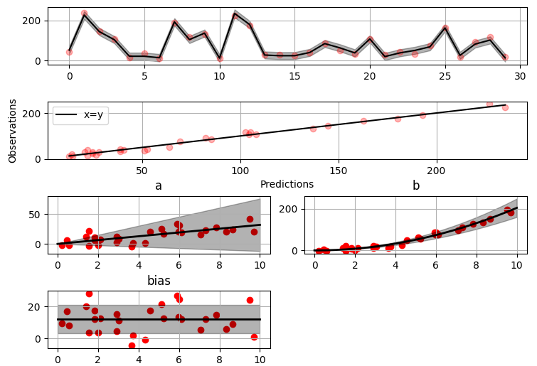 + +It is also possible to plot the estimated Γ-distribution of the noise precision +(inverse variance) as well as the 1-D Normal distributions of each individual +model parameter. + +Plot (prior or posterior) probability density functions of all model parameters: + +```python +>>> fig = gammy.plot.gaussian1d_density_plot(model) + +``` + +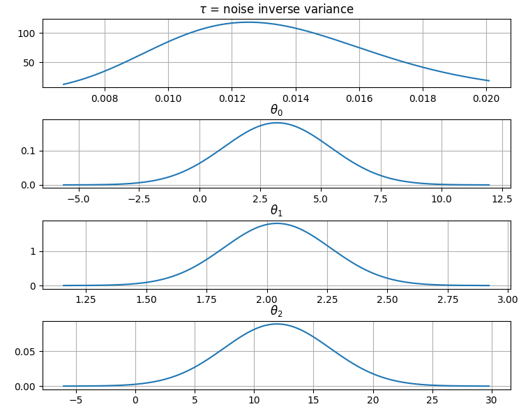 + +#### Saving model on hard disk + +Saving: + +<!-- NOTE: To skip doctests, one > has been removed --> +```python +>> model.save("/home/foobar/test.hdf5") +``` + +Loading: + +<!-- NOTE: To skip doctests, one > has been removed --> +```python +>> model = GAM(formula).load("/home/foobar/test.hdf5") +``` + +### Gaussian process regression + +Create fake dataset: + +```python +>>> n = 50 +>>> input_data = np.vstack((2 * np.pi * np.random.rand(n), np.random.rand(n))).T +>>> y = ( +... np.abs(np.cos(input_data[:, 0])) * input_data[:, 1] + +... 1 + 0.1 * np.random.randn(n) +... ) + +``` + +Define model: + +``` python +>>> a = gammy.formulae.ExpSineSquared1d( +... np.arange(0, 2 * np.pi, 0.1), +... corrlen=1.0, +... sigma=1.0, +... period=2 * np.pi, +... energy=0.99 +... ) +>>> bias = gammy.Scalar(prior=(0, 1e-6)) +>>> formula = a(x[:, 0]) * x[:, 1] + bias +>>> model = gammy.models.bayespy.GAM(formula).fit(input_data, y) + +>>> round(model.mean_theta[0][0], 8) +-0.8343458 + +``` + +Plot predictions and partial residuals: + +``` python +>>> fig = gammy.plot.validation_plot( +... model, +... input_data, +... y, +... grid_limits=[[0, 2 * np.pi], [0, 1]], +... input_maps=[x[:, 0:2], x[:, 1]], +... titles=["Surface estimate", "intercept"] +... ) + +``` + +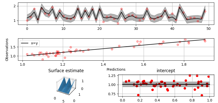 + +Plot parameter probability density functions + +``` python +>>> fig = gammy.plot.gaussian1d_density_plot(model) + +``` + +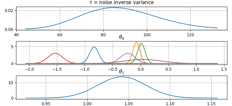 + +#### More covariance kernels + +The package contains covariance functions for many well-known options such as +the _Exponential squared_, _Periodic exponential squared_, _Rational quadratic_, +and the _Ornstein-Uhlenbeck_ kernels. Please see the documentation section [More +on Gaussian Process +kernels](https://malmgrek.github.io/gammy/features.html#more-on-gaussian-process-kernels) +for a gallery of kernels. + +#### Defining custom kernels + +Please read the documentation section: [Customize Gaussian Process +kernels](https://malmgrek.github.io/gammy/features.html#customize-gaussian-process-kernels) + +### Spline regression + +Constructing B-Spline based 1-D basis functions is also supported. Let's define +dummy data: + +```python +>>> n = 30 +>>> input_data = 10 * np.random.rand(n) +>>> y = 2.0 * input_data ** 2 + 7 + 10 * np.random.randn(n) + +``` + +Define model: + +``` python +>>> grid = np.arange(0, 11, 2.0) +>>> order = 2 +>>> N = len(grid) + order - 2 +>>> sigma = 10 ** 2 +>>> formula = gammy.BSpline1d( +... grid, +... order=order, +... prior=(np.zeros(N), np.identity(N) / sigma), +... extrapolate=True +... )(x) +>>> model = gammy.models.bayespy.GAM(formula).fit(input_data, y) + +>>> round(model.mean_theta[0][0], 8) +-49.00019115 + +``` + +Plot validation figure: + +``` python +>>> fig = gammy.plot.validation_plot( +... model, +... input_data, +... y, +... grid_limits=[-2, 12], +... input_maps=[x], +... titles=["a"] +... ) + +``` + +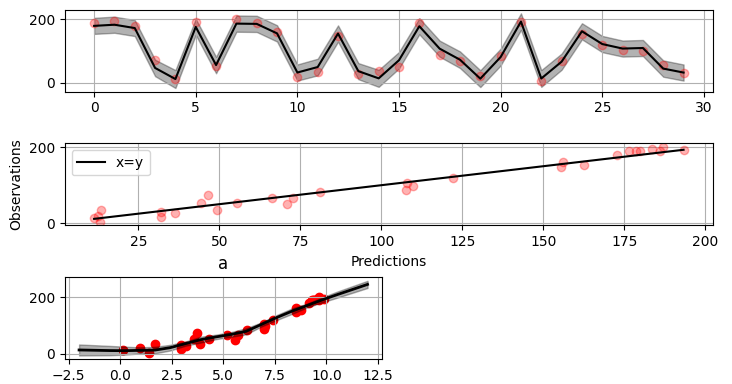 + +Plot parameter probability densities: + + ``` python +>>> fig = gammy.plot.gaussian1d_density_plot(model) + + ``` + +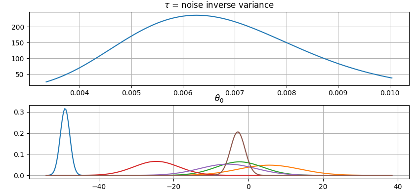 + +### Non-linear manifold regression + +In this example we try estimating the bivariate "MATLAB function" using a +Gaussian process model with Kronecker tensor structure (see e.g. +[PyMC3](https://docs.pymc.io/en/v3/pymc-examples/examples/gaussian_processes/GP-Kron.html)). The main point in the +below example is that it is quite straightforward to build models that can learn +arbitrary 2D-surfaces. + +Let us first create some artificial data using the MATLAB function! + +```python +>>> n = 100 +>>> input_data = np.vstack(( +... 6 * np.random.rand(n) - 3, 6 * np.random.rand(n) - 3 +... )).T +>>> y = ( +... gammy.utils.peaks(input_data[:, 0], input_data[:, 1]) + +... 4 + 0.3 * np.random.randn(n) +... ) + +``` + +There is support for forming two-dimensional basis functions given two +one-dimensional formulas. The new combined basis is essentially the outer +product of the given bases. The underlying weight prior distribution priors and +covariances are constructed using the Kronecker product. + +```python +>>> a = gammy.ExpSquared1d( +... np.arange(-3, 3, 0.1), +... corrlen=0.5, +... sigma=4.0, +... energy=0.99 +... )(x[:, 0]) # NOTE: Input map is defined here! +>>> b = gammy.ExpSquared1d( +... np.arange(-3, 3, 0.1), +... corrlen=0.5, +... sigma=4.0, +... energy=0.99 +... )(x[:, 1]) # NOTE: Input map is defined here! +>>> A = gammy.formulae.Kron(a, b) +>>> bias = gammy.formulae.Scalar(prior=(0, 1e-6)) +>>> formula = A + bias +>>> model = GAM(formula).fit(input_data, y) + +>>> round(model.mean_theta[0][0], 8) +0.37426986 + +``` + +Note that same logic could be used to construct higher dimensional bases, +that is, one could define a 3D-formula: + +<!-- NOTE: To skip doctests, one > has been removed --> +```python +>> formula_3d = gammy.Kron(gammy.Kron(a, b), c) + +``` + +Plot predictions and partial residuals: + +```python +>>> fig = gammy.plot.validation_plot( +... model, +... input_data, +... y, +... grid_limits=[[-3, 3], [-3, 3]], +... input_maps=[x, x[:, 0]], +... titles=["Surface estimate", "intercept"] +... ) + +``` + +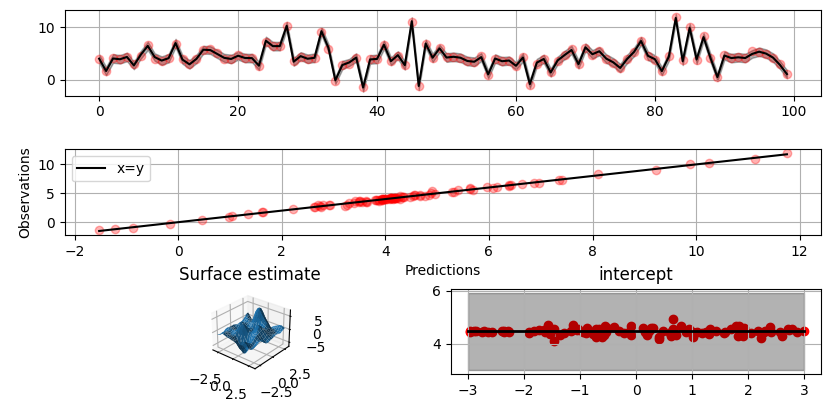 + +Plot parameter probability density functions: + +``` +>>> fig = gammy.plot.gaussian1d_density_plot(model) + +``` + +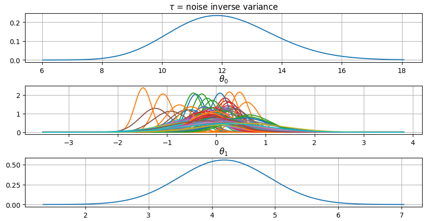 + +## Testing + +The package's unit tests can be ran with PyTest (`cd` to repository root): + +``` shell +pytest -v +``` + +Running this documentation as a Doctest: + +``` shell +python -m doctest -v README.md +``` + +## Package documentation + +Documentation of the package with code examples: +<https://malmgrek.github.io/gammy>. + + +%package -n python3-gammy +Summary: Generalized additive models with a Bayesian twist +Provides: python-gammy +BuildRequires: python3-devel +BuildRequires: python3-setuptools +BuildRequires: python3-pip +%description -n python3-gammy +# Gammy – Generalized additive models in Python with a Bayesian twist + + + +A Generalized additive model is a predictive mathematical model defined as a sum +of terms that are calibrated (fitted) with observation data. + +Generalized additive models form a surprisingly general framework for building +models for both production software and scientific research. This Python package +offers tools for building the model terms as decompositions of various basis +functions. It is possible to model the terms e.g. as Gaussian processes (with +reduced dimensionality) of various kernels, as piecewise linear functions, and +as B-splines, among others. Of course, very simple terms like lines and +constants are also supported (these are just very simple basis functions). + +The uncertainty in the weight parameter distributions is modeled using Bayesian +statistical analysis with the help of the superb package +[BayesPy](http://www.bayespy.org/index.html). Alternatively, it is possible to +fit models using just NumPy. + +<!-- markdown-toc start - Don't edit this section. Run M-x markdown-toc-refresh-toc --> +**Table of Contents** + +- [Installation](#installation) +- [Examples](#examples) + - [Polynomial regression on 'roids](#polynomial-regression-on-roids) + - [Predicting with model](#predicting-with-model) + - [Plotting results](#plotting-results) + - [Saving model on hard disk](#saving-model-on-hard-disk) + - [Gaussian process regression](#gaussian-process-regression) + - [More covariance kernels](#more-covariance-kernels) + - [Defining custom kernels](#defining-custom-kernels) + - [Spline regression](#spline-regression) + - [Non-linear manifold regression](#non-linear-manifold-regression) +- [Testing](#testing) +- [Package documentation](#package-documentation) + +<!-- markdown-toc end --> + +## Installation + +The package is found in PyPi. + +``` shell +pip install gammy +``` + +## Examples + +In this overview, we demonstrate the package's most important features through +common usage examples. + +### Polynomial regression on 'roids + +A typical simple (but sometimes non-trivial) modeling task is to estimate an +unknown function from noisy data. First we import the bare minimum dependencies to be used in the below examples: + +```python +>>> import numpy as np + +>>> import gammy +>>> from gammy.models.bayespy import GAM + +>>> gammy.__version__ +'0.5.0' + +``` + +Let's simulate a dataset: + +```python +>>> np.random.seed(42) + +>>> n = 30 +>>> input_data = 10 * np.random.rand(n) +>>> y = 5 * input_data + 2.0 * input_data ** 2 + 7 + 10 * np.random.randn(n) + +``` + +The object `x` is just a convenience tool for defining input data maps +as if they were just Numpy arrays: + +```python +>>> from gammy.arraymapper import x + +``` + +Define and fit the model: + +```python +>>> a = gammy.formulae.Scalar(prior=(0, 1e-6)) +>>> b = gammy.formulae.Scalar(prior=(0, 1e-6)) +>>> bias = gammy.formulae.Scalar(prior=(0, 1e-6)) +>>> formula = a * x + b * x ** 2 + bias +>>> model = GAM(formula).fit(input_data, y) + +``` + +The model attribute `model.theta` characterizes the Gaussian posterior +distribution of the model parameters vector. + +``` python +>>> model.mean_theta +[array([3.20130444]), array([2.0420961]), array([11.93437195])] + +``` + +Variance of additive zero-mean normally distributed noise is estimated +automagically: + +``` python +>>> round(model.inv_mean_tau, 8) +74.51660744 + +``` + +#### Predicting with model + +```python +>>> model.predict(input_data[:2]) +array([ 52.57112684, 226.9460579 ]) + +``` + +Predictions with uncertainty, that is, posterior predictive mean and variance +can be calculated as follows: + +```python +>>> model.predict_variance(input_data[:2]) +(array([ 52.57112684, 226.9460579 ]), array([79.35827362, 95.16358131])) + +``` + +#### Plotting results + +```python +>>> fig = gammy.plot.validation_plot( +... model, +... input_data, +... y, +... grid_limits=[0, 10], +... input_maps=[x, x, x], +... titles=["a", "b", "bias"] +... ) + +``` + +The grey band in the top figure is two times the prediction standard deviation +and, in the partial residual plots, two times the respective marginal posterior +standard deviation. + + + +It is also possible to plot the estimated Γ-distribution of the noise precision +(inverse variance) as well as the 1-D Normal distributions of each individual +model parameter. + +Plot (prior or posterior) probability density functions of all model parameters: + +```python +>>> fig = gammy.plot.gaussian1d_density_plot(model) + +``` + + + +#### Saving model on hard disk + +Saving: + +<!-- NOTE: To skip doctests, one > has been removed --> +```python +>> model.save("/home/foobar/test.hdf5") +``` + +Loading: + +<!-- NOTE: To skip doctests, one > has been removed --> +```python +>> model = GAM(formula).load("/home/foobar/test.hdf5") +``` + +### Gaussian process regression + +Create fake dataset: + +```python +>>> n = 50 +>>> input_data = np.vstack((2 * np.pi * np.random.rand(n), np.random.rand(n))).T +>>> y = ( +... np.abs(np.cos(input_data[:, 0])) * input_data[:, 1] + +... 1 + 0.1 * np.random.randn(n) +... ) + +``` + +Define model: + +``` python +>>> a = gammy.formulae.ExpSineSquared1d( +... np.arange(0, 2 * np.pi, 0.1), +... corrlen=1.0, +... sigma=1.0, +... period=2 * np.pi, +... energy=0.99 +... ) +>>> bias = gammy.Scalar(prior=(0, 1e-6)) +>>> formula = a(x[:, 0]) * x[:, 1] + bias +>>> model = gammy.models.bayespy.GAM(formula).fit(input_data, y) + +>>> round(model.mean_theta[0][0], 8) +-0.8343458 + +``` + +Plot predictions and partial residuals: + +``` python +>>> fig = gammy.plot.validation_plot( +... model, +... input_data, +... y, +... grid_limits=[[0, 2 * np.pi], [0, 1]], +... input_maps=[x[:, 0:2], x[:, 1]], +... titles=["Surface estimate", "intercept"] +... ) + +``` + + + +Plot parameter probability density functions + +``` python +>>> fig = gammy.plot.gaussian1d_density_plot(model) + +``` + + + +#### More covariance kernels + +The package contains covariance functions for many well-known options such as +the _Exponential squared_, _Periodic exponential squared_, _Rational quadratic_, +and the _Ornstein-Uhlenbeck_ kernels. Please see the documentation section [More +on Gaussian Process +kernels](https://malmgrek.github.io/gammy/features.html#more-on-gaussian-process-kernels) +for a gallery of kernels. + +#### Defining custom kernels + +Please read the documentation section: [Customize Gaussian Process +kernels](https://malmgrek.github.io/gammy/features.html#customize-gaussian-process-kernels) + +### Spline regression + +Constructing B-Spline based 1-D basis functions is also supported. Let's define +dummy data: + +```python +>>> n = 30 +>>> input_data = 10 * np.random.rand(n) +>>> y = 2.0 * input_data ** 2 + 7 + 10 * np.random.randn(n) + +``` + +Define model: + +``` python +>>> grid = np.arange(0, 11, 2.0) +>>> order = 2 +>>> N = len(grid) + order - 2 +>>> sigma = 10 ** 2 +>>> formula = gammy.BSpline1d( +... grid, +... order=order, +... prior=(np.zeros(N), np.identity(N) / sigma), +... extrapolate=True +... )(x) +>>> model = gammy.models.bayespy.GAM(formula).fit(input_data, y) + +>>> round(model.mean_theta[0][0], 8) +-49.00019115 + +``` + +Plot validation figure: + +``` python +>>> fig = gammy.plot.validation_plot( +... model, +... input_data, +... y, +... grid_limits=[-2, 12], +... input_maps=[x], +... titles=["a"] +... ) + +``` + + + +Plot parameter probability densities: + + ``` python +>>> fig = gammy.plot.gaussian1d_density_plot(model) + + ``` + + + +### Non-linear manifold regression + +In this example we try estimating the bivariate "MATLAB function" using a +Gaussian process model with Kronecker tensor structure (see e.g. +[PyMC3](https://docs.pymc.io/en/v3/pymc-examples/examples/gaussian_processes/GP-Kron.html)). The main point in the +below example is that it is quite straightforward to build models that can learn +arbitrary 2D-surfaces. + +Let us first create some artificial data using the MATLAB function! + +```python +>>> n = 100 +>>> input_data = np.vstack(( +... 6 * np.random.rand(n) - 3, 6 * np.random.rand(n) - 3 +... )).T +>>> y = ( +... gammy.utils.peaks(input_data[:, 0], input_data[:, 1]) + +... 4 + 0.3 * np.random.randn(n) +... ) + +``` + +There is support for forming two-dimensional basis functions given two +one-dimensional formulas. The new combined basis is essentially the outer +product of the given bases. The underlying weight prior distribution priors and +covariances are constructed using the Kronecker product. + +```python +>>> a = gammy.ExpSquared1d( +... np.arange(-3, 3, 0.1), +... corrlen=0.5, +... sigma=4.0, +... energy=0.99 +... )(x[:, 0]) # NOTE: Input map is defined here! +>>> b = gammy.ExpSquared1d( +... np.arange(-3, 3, 0.1), +... corrlen=0.5, +... sigma=4.0, +... energy=0.99 +... )(x[:, 1]) # NOTE: Input map is defined here! +>>> A = gammy.formulae.Kron(a, b) +>>> bias = gammy.formulae.Scalar(prior=(0, 1e-6)) +>>> formula = A + bias +>>> model = GAM(formula).fit(input_data, y) + +>>> round(model.mean_theta[0][0], 8) +0.37426986 + +``` + +Note that same logic could be used to construct higher dimensional bases, +that is, one could define a 3D-formula: + +<!-- NOTE: To skip doctests, one > has been removed --> +```python +>> formula_3d = gammy.Kron(gammy.Kron(a, b), c) + +``` + +Plot predictions and partial residuals: + +```python +>>> fig = gammy.plot.validation_plot( +... model, +... input_data, +... y, +... grid_limits=[[-3, 3], [-3, 3]], +... input_maps=[x, x[:, 0]], +... titles=["Surface estimate", "intercept"] +... ) + +``` + + + +Plot parameter probability density functions: + +``` +>>> fig = gammy.plot.gaussian1d_density_plot(model) + +``` + + + +## Testing + +The package's unit tests can be ran with PyTest (`cd` to repository root): + +``` shell +pytest -v +``` + +Running this documentation as a Doctest: + +``` shell +python -m doctest -v README.md +``` + +## Package documentation + +Documentation of the package with code examples: +<https://malmgrek.github.io/gammy>. + + +%package help +Summary: Development documents and examples for gammy +Provides: python3-gammy-doc +%description help +# Gammy – Generalized additive models in Python with a Bayesian twist + + + +A Generalized additive model is a predictive mathematical model defined as a sum +of terms that are calibrated (fitted) with observation data. + +Generalized additive models form a surprisingly general framework for building +models for both production software and scientific research. This Python package +offers tools for building the model terms as decompositions of various basis +functions. It is possible to model the terms e.g. as Gaussian processes (with +reduced dimensionality) of various kernels, as piecewise linear functions, and +as B-splines, among others. Of course, very simple terms like lines and +constants are also supported (these are just very simple basis functions). + +The uncertainty in the weight parameter distributions is modeled using Bayesian +statistical analysis with the help of the superb package +[BayesPy](http://www.bayespy.org/index.html). Alternatively, it is possible to +fit models using just NumPy. + +<!-- markdown-toc start - Don't edit this section. Run M-x markdown-toc-refresh-toc --> +**Table of Contents** + +- [Installation](#installation) +- [Examples](#examples) + - [Polynomial regression on 'roids](#polynomial-regression-on-roids) + - [Predicting with model](#predicting-with-model) + - [Plotting results](#plotting-results) + - [Saving model on hard disk](#saving-model-on-hard-disk) + - [Gaussian process regression](#gaussian-process-regression) + - [More covariance kernels](#more-covariance-kernels) + - [Defining custom kernels](#defining-custom-kernels) + - [Spline regression](#spline-regression) + - [Non-linear manifold regression](#non-linear-manifold-regression) +- [Testing](#testing) +- [Package documentation](#package-documentation) + +<!-- markdown-toc end --> + +## Installation + +The package is found in PyPi. + +``` shell +pip install gammy +``` + +## Examples + +In this overview, we demonstrate the package's most important features through +common usage examples. + +### Polynomial regression on 'roids + +A typical simple (but sometimes non-trivial) modeling task is to estimate an +unknown function from noisy data. First we import the bare minimum dependencies to be used in the below examples: + +```python +>>> import numpy as np + +>>> import gammy +>>> from gammy.models.bayespy import GAM + +>>> gammy.__version__ +'0.5.0' + +``` + +Let's simulate a dataset: + +```python +>>> np.random.seed(42) + +>>> n = 30 +>>> input_data = 10 * np.random.rand(n) +>>> y = 5 * input_data + 2.0 * input_data ** 2 + 7 + 10 * np.random.randn(n) + +``` + +The object `x` is just a convenience tool for defining input data maps +as if they were just Numpy arrays: + +```python +>>> from gammy.arraymapper import x + +``` + +Define and fit the model: + +```python +>>> a = gammy.formulae.Scalar(prior=(0, 1e-6)) +>>> b = gammy.formulae.Scalar(prior=(0, 1e-6)) +>>> bias = gammy.formulae.Scalar(prior=(0, 1e-6)) +>>> formula = a * x + b * x ** 2 + bias +>>> model = GAM(formula).fit(input_data, y) + +``` + +The model attribute `model.theta` characterizes the Gaussian posterior +distribution of the model parameters vector. + +``` python +>>> model.mean_theta +[array([3.20130444]), array([2.0420961]), array([11.93437195])] + +``` + +Variance of additive zero-mean normally distributed noise is estimated +automagically: + +``` python +>>> round(model.inv_mean_tau, 8) +74.51660744 + +``` + +#### Predicting with model + +```python +>>> model.predict(input_data[:2]) +array([ 52.57112684, 226.9460579 ]) + +``` + +Predictions with uncertainty, that is, posterior predictive mean and variance +can be calculated as follows: + +```python +>>> model.predict_variance(input_data[:2]) +(array([ 52.57112684, 226.9460579 ]), array([79.35827362, 95.16358131])) + +``` + +#### Plotting results + +```python +>>> fig = gammy.plot.validation_plot( +... model, +... input_data, +... y, +... grid_limits=[0, 10], +... input_maps=[x, x, x], +... titles=["a", "b", "bias"] +... ) + +``` + +The grey band in the top figure is two times the prediction standard deviation +and, in the partial residual plots, two times the respective marginal posterior +standard deviation. + + + +It is also possible to plot the estimated Γ-distribution of the noise precision +(inverse variance) as well as the 1-D Normal distributions of each individual +model parameter. + +Plot (prior or posterior) probability density functions of all model parameters: + +```python +>>> fig = gammy.plot.gaussian1d_density_plot(model) + +``` + + + +#### Saving model on hard disk + +Saving: + +<!-- NOTE: To skip doctests, one > has been removed --> +```python +>> model.save("/home/foobar/test.hdf5") +``` + +Loading: + +<!-- NOTE: To skip doctests, one > has been removed --> +```python +>> model = GAM(formula).load("/home/foobar/test.hdf5") +``` + +### Gaussian process regression + +Create fake dataset: + +```python +>>> n = 50 +>>> input_data = np.vstack((2 * np.pi * np.random.rand(n), np.random.rand(n))).T +>>> y = ( +... np.abs(np.cos(input_data[:, 0])) * input_data[:, 1] + +... 1 + 0.1 * np.random.randn(n) +... ) + +``` + +Define model: + +``` python +>>> a = gammy.formulae.ExpSineSquared1d( +... np.arange(0, 2 * np.pi, 0.1), +... corrlen=1.0, +... sigma=1.0, +... period=2 * np.pi, +... energy=0.99 +... ) +>>> bias = gammy.Scalar(prior=(0, 1e-6)) +>>> formula = a(x[:, 0]) * x[:, 1] + bias +>>> model = gammy.models.bayespy.GAM(formula).fit(input_data, y) + +>>> round(model.mean_theta[0][0], 8) +-0.8343458 + +``` + +Plot predictions and partial residuals: + +``` python +>>> fig = gammy.plot.validation_plot( +... model, +... input_data, +... y, +... grid_limits=[[0, 2 * np.pi], [0, 1]], +... input_maps=[x[:, 0:2], x[:, 1]], +... titles=["Surface estimate", "intercept"] +... ) + +``` + + + +Plot parameter probability density functions + +``` python +>>> fig = gammy.plot.gaussian1d_density_plot(model) + +``` + + + +#### More covariance kernels + +The package contains covariance functions for many well-known options such as +the _Exponential squared_, _Periodic exponential squared_, _Rational quadratic_, +and the _Ornstein-Uhlenbeck_ kernels. Please see the documentation section [More +on Gaussian Process +kernels](https://malmgrek.github.io/gammy/features.html#more-on-gaussian-process-kernels) +for a gallery of kernels. + +#### Defining custom kernels + +Please read the documentation section: [Customize Gaussian Process +kernels](https://malmgrek.github.io/gammy/features.html#customize-gaussian-process-kernels) + +### Spline regression + +Constructing B-Spline based 1-D basis functions is also supported. Let's define +dummy data: + +```python +>>> n = 30 +>>> input_data = 10 * np.random.rand(n) +>>> y = 2.0 * input_data ** 2 + 7 + 10 * np.random.randn(n) + +``` + +Define model: + +``` python +>>> grid = np.arange(0, 11, 2.0) +>>> order = 2 +>>> N = len(grid) + order - 2 +>>> sigma = 10 ** 2 +>>> formula = gammy.BSpline1d( +... grid, +... order=order, +... prior=(np.zeros(N), np.identity(N) / sigma), +... extrapolate=True +... )(x) +>>> model = gammy.models.bayespy.GAM(formula).fit(input_data, y) + +>>> round(model.mean_theta[0][0], 8) +-49.00019115 + +``` + +Plot validation figure: + +``` python +>>> fig = gammy.plot.validation_plot( +... model, +... input_data, +... y, +... grid_limits=[-2, 12], +... input_maps=[x], +... titles=["a"] +... ) + +``` + + + +Plot parameter probability densities: + + ``` python +>>> fig = gammy.plot.gaussian1d_density_plot(model) + + ``` + + + +### Non-linear manifold regression + +In this example we try estimating the bivariate "MATLAB function" using a +Gaussian process model with Kronecker tensor structure (see e.g. +[PyMC3](https://docs.pymc.io/en/v3/pymc-examples/examples/gaussian_processes/GP-Kron.html)). The main point in the +below example is that it is quite straightforward to build models that can learn +arbitrary 2D-surfaces. + +Let us first create some artificial data using the MATLAB function! + +```python +>>> n = 100 +>>> input_data = np.vstack(( +... 6 * np.random.rand(n) - 3, 6 * np.random.rand(n) - 3 +... )).T +>>> y = ( +... gammy.utils.peaks(input_data[:, 0], input_data[:, 1]) + +... 4 + 0.3 * np.random.randn(n) +... ) + +``` + +There is support for forming two-dimensional basis functions given two +one-dimensional formulas. The new combined basis is essentially the outer +product of the given bases. The underlying weight prior distribution priors and +covariances are constructed using the Kronecker product. + +```python +>>> a = gammy.ExpSquared1d( +... np.arange(-3, 3, 0.1), +... corrlen=0.5, +... sigma=4.0, +... energy=0.99 +... )(x[:, 0]) # NOTE: Input map is defined here! +>>> b = gammy.ExpSquared1d( +... np.arange(-3, 3, 0.1), +... corrlen=0.5, +... sigma=4.0, +... energy=0.99 +... )(x[:, 1]) # NOTE: Input map is defined here! +>>> A = gammy.formulae.Kron(a, b) +>>> bias = gammy.formulae.Scalar(prior=(0, 1e-6)) +>>> formula = A + bias +>>> model = GAM(formula).fit(input_data, y) + +>>> round(model.mean_theta[0][0], 8) +0.37426986 + +``` + +Note that same logic could be used to construct higher dimensional bases, +that is, one could define a 3D-formula: + +<!-- NOTE: To skip doctests, one > has been removed --> +```python +>> formula_3d = gammy.Kron(gammy.Kron(a, b), c) + +``` + +Plot predictions and partial residuals: + +```python +>>> fig = gammy.plot.validation_plot( +... model, +... input_data, +... y, +... grid_limits=[[-3, 3], [-3, 3]], +... input_maps=[x, x[:, 0]], +... titles=["Surface estimate", "intercept"] +... ) + +``` + + + +Plot parameter probability density functions: + +``` +>>> fig = gammy.plot.gaussian1d_density_plot(model) + +``` + + + +## Testing + +The package's unit tests can be ran with PyTest (`cd` to repository root): + +``` shell +pytest -v +``` + +Running this documentation as a Doctest: + +``` shell +python -m doctest -v README.md +``` + +## Package documentation + +Documentation of the package with code examples: +<https://malmgrek.github.io/gammy>. + + +%prep +%autosetup -n gammy-0.5.0 + +%build +%py3_build + +%install +%py3_install +install -d -m755 %{buildroot}/%{_pkgdocdir} +if [ -d doc ]; then cp -arf doc %{buildroot}/%{_pkgdocdir}; fi +if [ -d docs ]; then cp -arf docs %{buildroot}/%{_pkgdocdir}; fi +if [ -d example ]; then cp -arf example %{buildroot}/%{_pkgdocdir}; fi +if [ -d examples ]; then cp -arf examples %{buildroot}/%{_pkgdocdir}; fi +pushd %{buildroot} +if [ -d usr/lib ]; then + find usr/lib -type f -printf "/%h/%f\n" >> filelist.lst +fi +if [ -d usr/lib64 ]; then + find usr/lib64 -type f -printf "/%h/%f\n" >> filelist.lst +fi +if [ -d usr/bin ]; then + find usr/bin -type f -printf "/%h/%f\n" >> filelist.lst +fi +if [ -d usr/sbin ]; then + find usr/sbin -type f -printf "/%h/%f\n" >> filelist.lst +fi +touch doclist.lst +if [ -d usr/share/man ]; then + find usr/share/man -type f -printf "/%h/%f.gz\n" >> doclist.lst +fi +popd +mv %{buildroot}/filelist.lst . +mv %{buildroot}/doclist.lst . + +%files -n python3-gammy -f filelist.lst +%dir %{python3_sitelib}/* + +%files help -f doclist.lst +%{_docdir}/* + +%changelog +* Thu May 18 2023 Python_Bot <Python_Bot@openeuler.org> - 0.5.0-1 +- Package Spec generated @@ -0,0 +1 @@ +6096d6924ee927e10d06dc16357970ee gammy-0.5.0.tar.gz |