
diff options
| author | CoprDistGit <infra@openeuler.org> | 2023-05-18 05:24:10 +0000 |
|---|---|---|
| committer | CoprDistGit <infra@openeuler.org> | 2023-05-18 05:24:10 +0000 |
| commit | 6809070971efd65bc827f7b9ca6872312fde0489 (patch) | |
| tree | f30689a9bd58810b07682cbbca455732c5801089 | |
| parent | 2e7230e7dcc05502c7672fac8dfed699cc7b92ad (diff) | |
automatic import of python-geospacelab
| -rw-r--r-- | .gitignore | 1 | ||||
| -rw-r--r-- | python-geospacelab.spec | 1370 | ||||
| -rw-r--r-- | sources | 1 |
3 files changed, 1372 insertions, 0 deletions
@@ -0,0 +1 @@ +/geospacelab-0.6.1.tar.gz diff --git a/python-geospacelab.spec b/python-geospacelab.spec new file mode 100644 index 0000000..1429fbf --- /dev/null +++ b/python-geospacelab.spec @@ -0,0 +1,1370 @@ +%global _empty_manifest_terminate_build 0 +Name: python-geospacelab +Version: 0.6.1 +Release: 1 +Summary: Collect, manage, and visualize geospace data. +License: BSD 3-Clause License +URL: https://github.com/JouleCai/geospacelab +Source0: https://mirrors.nju.edu.cn/pypi/web/packages/f1/f2/bbb855019c19dcb5067b75e247236f991198dc5a13f299adee49806ce453/geospacelab-0.6.1.tar.gz +BuildArch: noarch + +Requires: python3-cython +Requires: python3-requests +Requires: python3-beautifulsoup4 +Requires: python3-natsort +Requires: python3-numpy +Requires: python3-scipy +Requires: python3-h5py +Requires: python3-netcdf4 +Requires: python3-matplotlib +Requires: python3-madrigalweb +Requires: python3-aacgmv2 +Requires: python3-cdflib +Requires: python3-geopack +Requires: python3-palettable +Requires: python3-toml +Requires: python3-sscws +Requires: python3-pandas + +%description +<p align="center"> + <img width="500" src="https://github.com/JouleCai/geospacelab/blob/master/docs/images/logo_v1_landscape_accent_colors.png"> +</p> + +# GeospaceLAB (geospacelab) +[](https://opensource.org/licenses/BSD-3-Clause) +[](https://www.python.org/) +[](https://zenodo.org/badge/latestdoi/347315860) +[](https://pepy.tech/project/geospacelab) + +[](https://pypi.python.org/pypi/geospacelab/) + + +GeospaceLAB provides a framework of data access, analysis, and visualization for the researchers in space physics and space weather. The documentation can be found +on [readthedocs.io](https://geospacelab.readthedocs.io/en/latest/). + +## Features +- Class-based data manager, including + - __DataHub__: the core module (top-level class) to manage data from multiple sources, + - __Dataset__: the middle-level class to download, load, and process data from a data source, + - __Variable__: the base-level class to store the data array of a variable with various attributes, including its + error, name, label, unit, group, and dependencies. +- Extendable + - Provide a standard procedure from downloading, loading, and post-processing the data. + - Easy to extend for a data source which has not been supported in the package. + - Flexible to add functions for post-processing. +- Visualization + - Time series plots with + - automatically adjustable time ticks and tick labels. + - dynamical panels (flexible to add or remove panels). + - automatically detect the time gaps. + - useful marking tools (vertical line crossing panels, shadings, top bars, etc, see Example 2 in +[Usage](https://github.com/JouleCai/geospacelab#usage)) + - Map projection + - Polar views with + - coastlines in either GEO or AACGM (APEX) coordinate system. + - mapping in either fixed lon/mlon mode or in fixed LST/MLT mode. + - Support 1-D or 2-D plots with + - satellite tracks (time ticks and labels) + - nadir colored 1-D plots + - gridded surface plots +- Space coordinate system transformation + - Unified interface for cs transformations. +- Toolboxes for data analysis + - Basic toolboxes for numpy array, datetime, logging, python dict, list, and class. + +## Built-in data sources: +| Data Source | Variables | File Format | Downloadable | Express | Status | +|-----------------------------|------------------------------------|-----------------------|---------------|-----------------|--------| +| CDAWeb/OMNI | Solar wind and IMF |*cdf* | *True* | __OMNIDashboard__ | stable | +| Madrigal/EISCAT | Ionospheric Ne, Te, Ti, ... | *EISCAT-hdf5*, *Madrigal-hdf5* | *True* | __EISCATDashboard__ | stable | +| Madrigal/GNSS/TECMAP | Ionospheric GPS TEC map | *hdf5* | *True* | - | beta | +| Madrigal/DMSP/s1 | DMSP SSM, SSIES, etc | *hdf5* | *True* | __DMSPTSDashboard__ | stable | +| Madrigal/DMSP/s4 | DMSP SSIES | *hdf5* | *True* | __DMSPTSDashboard__ | stable | +| Madrigal/DMSP/e | DMSP SSJ | *hdf5* | *True* | __DMSPTSDashboard__ | stable | +| Madrigal/Millstone Hill ISR | Millstone Hill ISR | *hdf5* | *True* | __MillstoneHillISRDashboard__ | stable | +| JHUAPL/DMSP/SSUSI | DMSP SSUSI | *netcdf* | *True* | __DMSPSSUSIDashboard__ | stable | +| JHUAPL/AMPERE/fitted | AMPERE FAC | *netcdf* | *False* | __AMPEREDashboard__ | stable | +| SuperDARN/POTMAP | SuperDARN potential map | *ascii* | *False* | - | stable | +| WDC/Dst | Dst index | *IAGA2002-ASCII* | *True* | - | stable | +| WDC/ASYSYM | ASY/SYM indices | *IAGA2002-ASCII* | *True* | __OMNIDashboard__ | stable | +| WDC/AE | AE indices | *IAGA2002-ASCII* | *True* | __OMNIDashboard__ | stable | +| GFZ/Kp | Kp/Ap indices | *ASCII* | *True* | - | stable | +| GFZ/Hpo | Hp30 or Hp60 indices | *ASCII* | *True* | - | stable | +| GFZ/SNF107 | SN, F107 | *ASCII* | *True* | - | stable | +| ESA/SWARM/EFI_LP_HM | SWARM Ne, Te, etc. | *netcdf* | *True* | - | stable | +| ESA/SWARM/EFI_TCT02 | SWARM cross track vi | *netcdf* | *True* | - | stable | +| ESA/SWARM/AOB_FAC_2F | SWARM FAC, auroral oval boundary | *netcdf* | *True* | - | beta | +| TUDelft/SWARM/DNS_POD | Swarm $\rho_n$ (GPS derived) | *ASCII* | *True* | - | stable | +| TUDelft/SWARM/DNS_ACC | Swarm $\rho_n$ (GPS+Accelerometer) | *ASCII* | *True* | - | stable | +| TUDelft/GOCE/WIND_ACC | GOCE neutral wind | *ASCII* | *True* | - | stable | +| TUDelft/GRACE/WIND_ACC | GRACE neutral wind | *ASCII* | *True* | - | stable | +| TUDelft/GRACE/DNS_ACC | Grace $\rho_n$ | *ASCII* | *True* | - | stable | +| TUDelft/CHAMP/DNS_ACC | CHAMP $\rho_n$ | *ASCII* | *True* | - | stable | + | UTA/GITM/2DALL | GITM 2D output | *binary*, *IDL-sav* | *False* | - | beta | + | UTA/GITM/3DALL | GITM 3D output | *binary*, *IDL-sav* | *False* | - | beta | + + + +## Installation +### 1. The python distribution "*__Anaconda__*" is recommended: +The package was tested with the anaconda distribution and with **PYTHON>=3.7** under **Ubuntu 20.04** and **MacOS Big Sur**. + +With Anaconda, it may be easier to install some required dependencies listed below, e.g., cartopy, using the _conda_ command. +It's also recommended installing the package and dependencies in a virtual environment with anaconda. + +After [installing the anaconda distribution](https://docs.anaconda.com/anaconda/install/index.html), a virtual environment can be created by the code below in the terminal: + +```shell +conda create --name [YOUR_ENV_NAME] -c conda-forge python cython cartopy +``` +The package "spyder" is a widely-used python IDE. Other IDEs, like "VS Code" or "Pycharm" also work. + +> **_Note:_** The recommended IDE is Spyder. Sometimes, a *RuntimeError* can be raised +> when the __aacgmv2__ package is called in **PyCharm** or **VS Code**. +> If you meet this issue, try to compile the codes in **Spyder** several times. + +After creating the virtual environement, you need to activate the virtual environment: + +```shell +conda activate [YOUR_ENV_NAME] +``` +and then to install the package as shown below or to start the IDE **Spyder**. + +More detailed information to set the anaconda environment can be found [here](https://conda.io/projects/conda/en/latest/user-guide/tasks/manage-environments.html#), + +### 2. Installation +#### Quick install from the pre-built release (recommended): +```shell +pip install geospacelab +``` + +#### Install from [Github](https://github.com/JouleCai/geospacelab) (not recommended): +```shell +pip install git+https://github.com/JouleCai/geospacelab@master +``` + +### 2. Dependencies +The package dependencies need to be installed before or after the installation of the package. +Several dependencies will be installed automatically with the package installation, +including __toml__, __requests__, __bueatifulsoup4__, __numpy__, __scipy__, __matplotlib__, __h5py__, __netcdf4__, +__cdflib__, __madrigalweb__, __sscws__, and __aacgmv2__. + +Other dependencies will be needed if you see a *__ImportError__* or *__ModuleNotFoundError__* +displayed in the python console. Some frequently used modules and their installation methods are listed below: +- [__cartopy__](https://scitools.org.uk/cartopy/docs/latest/installing.html): Map projection for geospatial data. + - ```conda install -c conda-forge cartopy ``` +- [__apexpy__ \*](https://apexpy.readthedocs.io/en/latest/reference/Apex.html): Apex and Quasi-Dipole geomagnetic +coordinate system. + - ```pip install apexpy ``` +- [__geopack__](https://github.com/tsssss/geopack): The geopack and Tsyganenko models in Python. + - ```pip install geopack ``` + +> ([\*]()): The **_gcc_** or **_gfortran_** compilers are required before installing the package. +> - gcc: ```conda install -c conda-forge gcc``` +> - gfortran: ```conda install -c conda-forge gfortran ``` + +Please install the packages above, if needed. + +Note: The package is currently pre-released. The installation methods may be changed in the future. + + +### 4. First-time startup and basic configuration +Some basic configurations will be made with the first-time import of the package. Following the messages prompted in the python console, the first configuration is to set the root directory for storing the data. + +When the modules to access the online Madrigal database is imported, it will ask for the inputs of user's full name, email, and affiliation. + +The user's configuration can be found from the *__toml__* file below: +``` +[your_home_directory]/.geospacelab/config.toml +``` +The user can set or change the preferences in the configuration file. For example, to change the root directory for storing the data, modify or add the lines in "config.toml": +```toml +[datahub] +data_root_dir = "YOUR_ROOT_DIR" +``` +To set the Madrigal cookies, change the lines: +```toml +[datahub.madrigal] +user_fullname = "YOUR_NAME" +user_email = "YOU_EMAIL" +user_affiliation = "YOUR_AFFILIATION" +``` + +### 5. Upgrade + +If the package is installed from the pre-built release. Update the package via: +```shell +pip install geospacelab --upgrade +``` + +### 6. Uninstallation +Uninstall the package via: +```shell +pip uninstall geospacelab +``` +If you don't need the user's configuration, delete the file at **_[your_home_directory]/.geospacelab/config.toml_** + +## Usage +### Example 1: Dock a sourced dataset and get variables: +The core of the data manager is the class Datahub. A Datahub instance will be used for docking a buit-in sourced dataset, or adding a temporary or user-defined dataset. + +The "dataset" is a Dataset instance, which is used for loading and downloading +the data. + +Below is an example to load the EISCAT data from the online service. The module will download EISCAT data automatically from +[the EISCAT schedule page](https://portal.eiscat.se/schedule/) with the presetttings of loading mode "AUTO" and file type "eiscat-hdf5". + +Example 1: +```python +import datetime + +from geospacelab.datahub import DataHub + +# settings +dt_fr = datetime.datetime.strptime('20210309' + '0000', '%Y%m%d%H%M') # datetime from +dt_to = datetime.datetime.strptime('20210309' + '2359', '%Y%m%d%H%M') # datetime to +database_name = 'madrigal' # built-in sourced database name +facility_name = 'eiscat' # facility name + +site = 'UHF' # facility attributes required, check from the eiscat schedule page +antenna = 'UHF' +modulation = 'ant' + +# create a datahub instance +dh = DataHub(dt_fr, dt_to) +# dock the first dataset (dataset index starts from 0) +ds_isr = dh.dock(datasource_contents=[database_name, 'isr', facility_name], + site=site, antenna=antenna, modulation=modulation, data_file_type='eiscat-hdf5') +# load data +ds_isr.load_data() +# assign a variable from its own dataset to the datahub +n_e = dh.assign_variable('n_e') +T_i = dh.assign_variable('T_i') + +# get the variables which have been assigned in the datahub +n_e = dh.get_variable('n_e') +T_i = dh.get_variable('T_i') +# if the variable is not assigned in the datahub, but exists in the its own dataset: +comp_O_p = dh.get_variable('comp_O_p', dataset=ds_isr) # O+ ratio +# above line is equivalent to +comp_O_p = dh.datasets[0]['comp_O_p'] + +# The variables, e.g., n_e and T_i, are the class Variable's instances, +# which stores the variable values, errors, and many other attributes, e.g., name, label, unit, depends, .... +# To get the value of the variable, use variable_isntance.value, e.g., +print(n_e.value) # return the variable's value, type: numpy.ndarray, axis 0 is always along the time, check n_e.depends.items{} +print(n_e.error) + +``` + +### Example 2: EISCAT quicklook plot +The EISCAT quicklook plot shows the GUISDAP analysed results in the same format as the online EISCAT quicklook plot. +The figure layout and quality are improved. In addition, several marking tools like vertical lines, shadings, top bars can be +added in the plot. See the example script and figure below: + +In "example2.py" +```python +import datetime +import geospacelab.express.eiscat_dashboard as eiscat + +dt_fr = datetime.datetime.strptime('20201209' + '1800', '%Y%m%d%H%M') +dt_to = datetime.datetime.strptime('20201210' + '0600', '%Y%m%d%H%M') + +site = 'UHF' +antenna = 'UHF' +modulation = '60' +load_mode = 'AUTO' +dashboard = eiscat.EISCATDashboard( + dt_fr, dt_to, site=site, antenna=antenna, modulation=modulation, load_mode='AUTO' +) +dashboard.quicklook() + +# dashboard.save_figure() # comment this if you need to run the following codes +# dashboard.show() # comment this if you need to run the following codes. + +""" +As the dashboard class (EISCATDashboard) is a inheritance of the classes Datahub and TSDashboard. +The variables can be retrieved in the same ways as shown in Example 1. +""" +n_e = dashboard.assign_variable('n_e') +print(n_e.value) +print(n_e.error) + +""" +Several marking tools (vertical lines, shadings, and top bars) can be added as the overlays +on the top of the quicklook plot. +""" +# add vertical line +dt_fr_2 = datetime.datetime.strptime('20201209' + '2030', "%Y%m%d%H%M") +dt_to_2 = datetime.datetime.strptime('20201210' + '0130', "%Y%m%d%H%M") +dashboard.add_vertical_line(dt_fr_2, bottom_extend=0, top_extend=0.02, label='Line 1', label_position='top') +# add shading +dashboard.add_shading(dt_fr_2, dt_to_2, bottom_extend=0, top_extend=0.02, label='Shading 1', label_position='top') +# add top bar +dt_fr_3 = datetime.datetime.strptime('20201210' + '0130', "%Y%m%d%H%M") +dt_to_3 = datetime.datetime.strptime('20201210' + '0430', "%Y%m%d%H%M") +dashboard.add_top_bar(dt_fr_3, dt_to_3, bottom=0., top=0.02, label='Top bar 1') + +# save figure +dashboard.save_figure() +# show on screen +dashboard.show() +``` +Output: +> 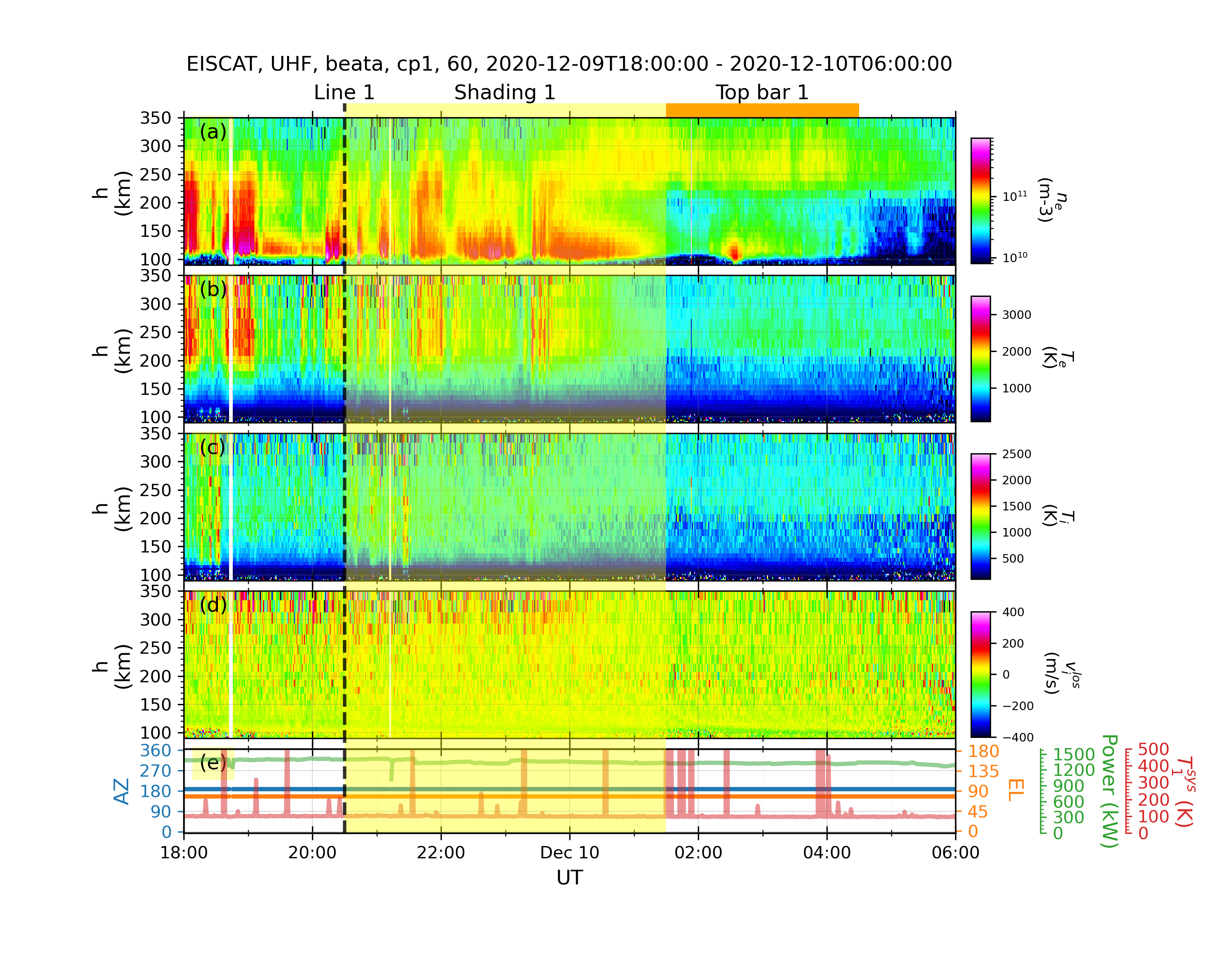 + +### Example 3: OMNI data and geomagnetic indices (WDC + GFZ): + +In "example3.py" + +```python +import datetime +import geospacelab.express.omni_dashboard as omni + +dt_fr = datetime.datetime.strptime('20160314' + '0600', '%Y%m%d%H%M') +dt_to = datetime.datetime.strptime('20160320' + '0600', '%Y%m%d%H%M') + +omni_type = 'OMNI2' +omni_res = '1min' +load_mode = 'AUTO' +dashboard = omni.OMNIDashboard( + dt_fr, dt_to, omni_type=omni_type, omni_res=omni_res, load_mode=load_mode +) +dashboard.quicklook() + +# data can be retrieved in the same way as in Example 1: +dashboard.list_assigned_variables() +B_x_gsm = dashboard.get_variable('B_x_GSM', dataset_index=0) +# save figure +dashboard.save_figure() +# show on screen +dashboard.show() +``` +Output: +> 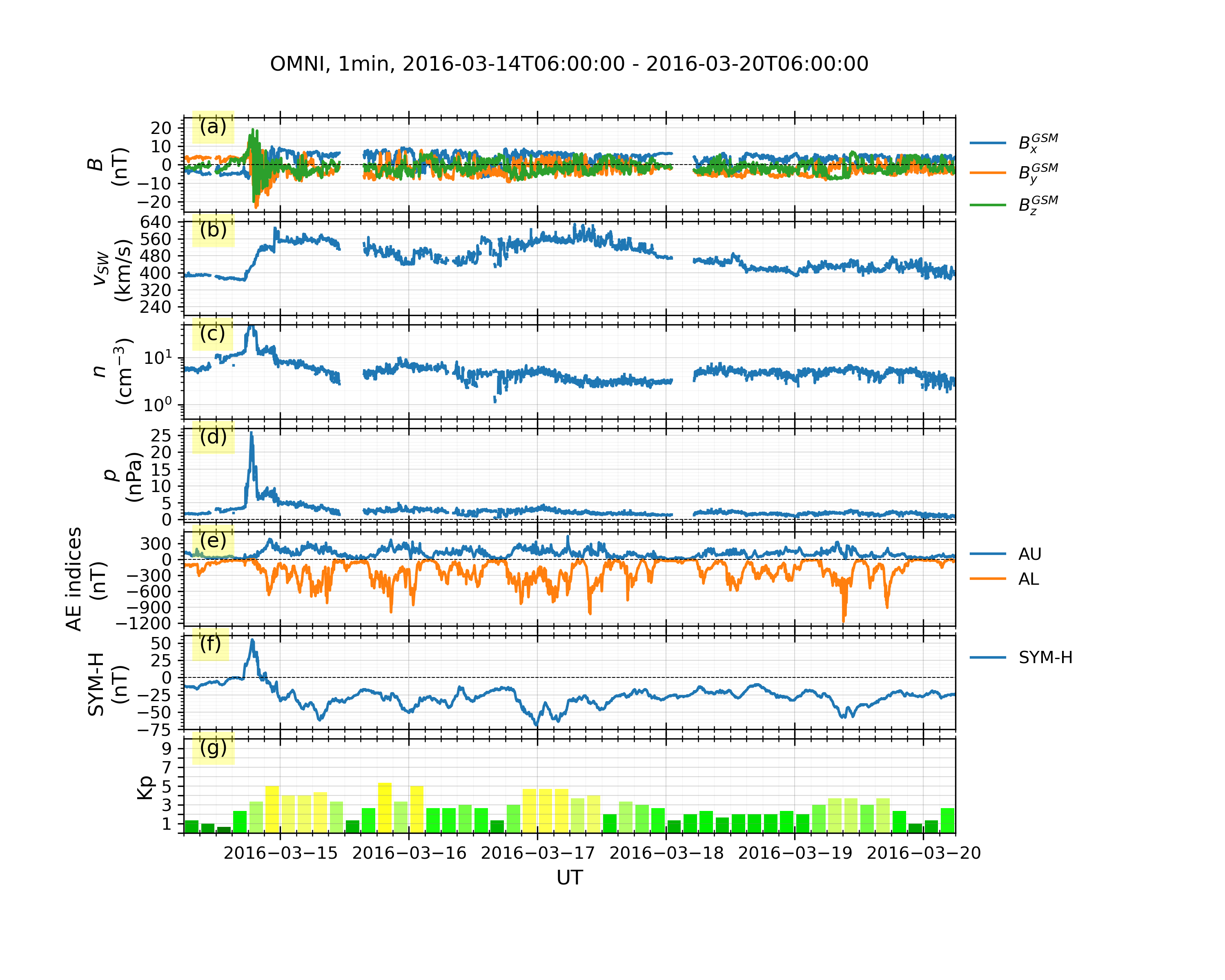 + +### Example 4: Mapping geospatial data in the polar map. +```python +import datetime +import matplotlib.pyplot as plt + +import geospacelab.visualization.mpl.geomap.geodashboards as geomap + +dt_fr = datetime.datetime(2015, 9, 8, 8) +dt_to = datetime.datetime(2015, 9, 8, 23, 59) +time1 = datetime.datetime(2015, 9, 8, 20, 21) +pole = 'N' +sat_id = 'f16' +band = 'LBHS' + +# Create a geodashboard object +dashboard = geomap.GeoDashboard(dt_fr=dt_fr, dt_to=dt_to, figure_config={'figsize': (5, 5)}) + +# If the orbit_id is specified, only one file will be downloaded. This option saves the downloading time. +# dashboard.dock(datasource_contents=['jhuapl', 'dmsp', 'ssusi', 'edraur'], pole='N', sat_id='f17', orbit_id='46863') +# If not specified, the data during the whole day will be downloaded. +dashboard.dock(datasource_contents=['jhuapl', 'dmsp', 'ssusi', 'edraur'], pole=pole, sat_id=sat_id, orbit_id=None) +ds_s1 = dashboard.dock( + datasource_contents=['madrigal', 'satellites', 'dmsp', 's1'], + dt_fr=time1 - datetime.timedelta(minutes=45), + dt_to=time1 + datetime.timedelta(minutes=45), + sat_id=sat_id) + +dashboard.set_layout(1, 1) + +# Get the variables: LBHS emission intensiy, corresponding times and locations +lbhs = dashboard.assign_variable('GRID_AUR_' + band, dataset_index=0) +dts = dashboard.assign_variable('DATETIME', dataset_index=0).value.flatten() +mlat = dashboard.assign_variable('GRID_MLAT', dataset_index=0).value +mlon = dashboard.assign_variable('GRID_MLON', dataset_index=0).value +mlt = dashboard.assign_variable(('GRID_MLT'), dataset_index=0).value + +# Search the index for the time to plot, used as an input to the following polar map +ind_t = dashboard.datasets[0].get_time_ind(ut=time1) +lbhs_ = lbhs.value[ind_t] +mlat_ = mlat[ind_t] +mlon_ = mlon[ind_t] +mlt_ = mlt[ind_t] +# Add a polar map panel to the dashboard. Currently the style is the fixed MLT at mlt_c=0. See the keywords below: +panel1 = dashboard.add_polar_map(row_ind=0, col_ind=0, style='mlt-fixed', cs='AACGM', mlt_c=0., pole=pole, ut=time1, boundary_lat=65., mirror_south=True) + +# Some settings for plotting. +pcolormesh_config = lbhs.visual.plot_config.pcolormesh +# Overlay the SSUSI image in the map. +ipm = panel1.overlay_pcolormesh(data=lbhs_, coords={'lat': mlat_, 'lon': mlon_, 'mlt': mlt_}, cs='AACGM', + regridding=True, **pcolormesh_config) +# Add a color bar +panel1.add_colorbar(ipm, c_label=band + " (R)", c_scale=pcolormesh_config['c_scale'], left=1.1, bottom=0.1, + width=0.05, height=0.7) + +# Overlay the gridlines +panel1.overlay_gridlines(lat_res=5, lon_label_separator=5) + +# Overlay the coastlines in the AACGM coordinate +panel1.overlay_coastlines() + +# Overlay cross-track velocity along satellite trajectory +sc_dt = ds_s1['SC_DATETIME'].value.flatten() +sc_lat = ds_s1['SC_GEO_LAT'].value.flatten() +sc_lon = ds_s1['SC_GEO_LON'].value.flatten() +sc_alt = ds_s1['SC_GEO_ALT'].value.flatten() +sc_coords = {'lat': sc_lat, 'lon': sc_lon, 'height': sc_alt} + +v_H = ds_s1['v_i_H'].value.flatten() +panel1.overlay_cross_track_vector(vector=v_H, unit_vector=1000, alpha=0.5, color='r', sc_coords=sc_coords, sc_ut=sc_dt, cs='GEOC') +# Overlay the satellite trajectory with ticks +panel1.overlay_sc_trajectory(sc_ut=sc_dt, sc_coords=sc_coords, cs='GEOC') + +# Add the title and save the figure +polestr = 'North' if pole == 'N' else 'South' +panel1.add_title(title='DMSP/SSUSI, ' + band + ', ' + sat_id.upper() + ', ' + polestr + ', ' + time1.strftime('%Y-%m-%d %H%M UT')) +plt.savefig('DMSP_SSUSI_' + time1.strftime('%Y%m%d-%H%M') + '_' + band + '_' + sat_id.upper() + '_' + pole, dpi=300) + +# show the figure +plt.show() +``` +Output: +> 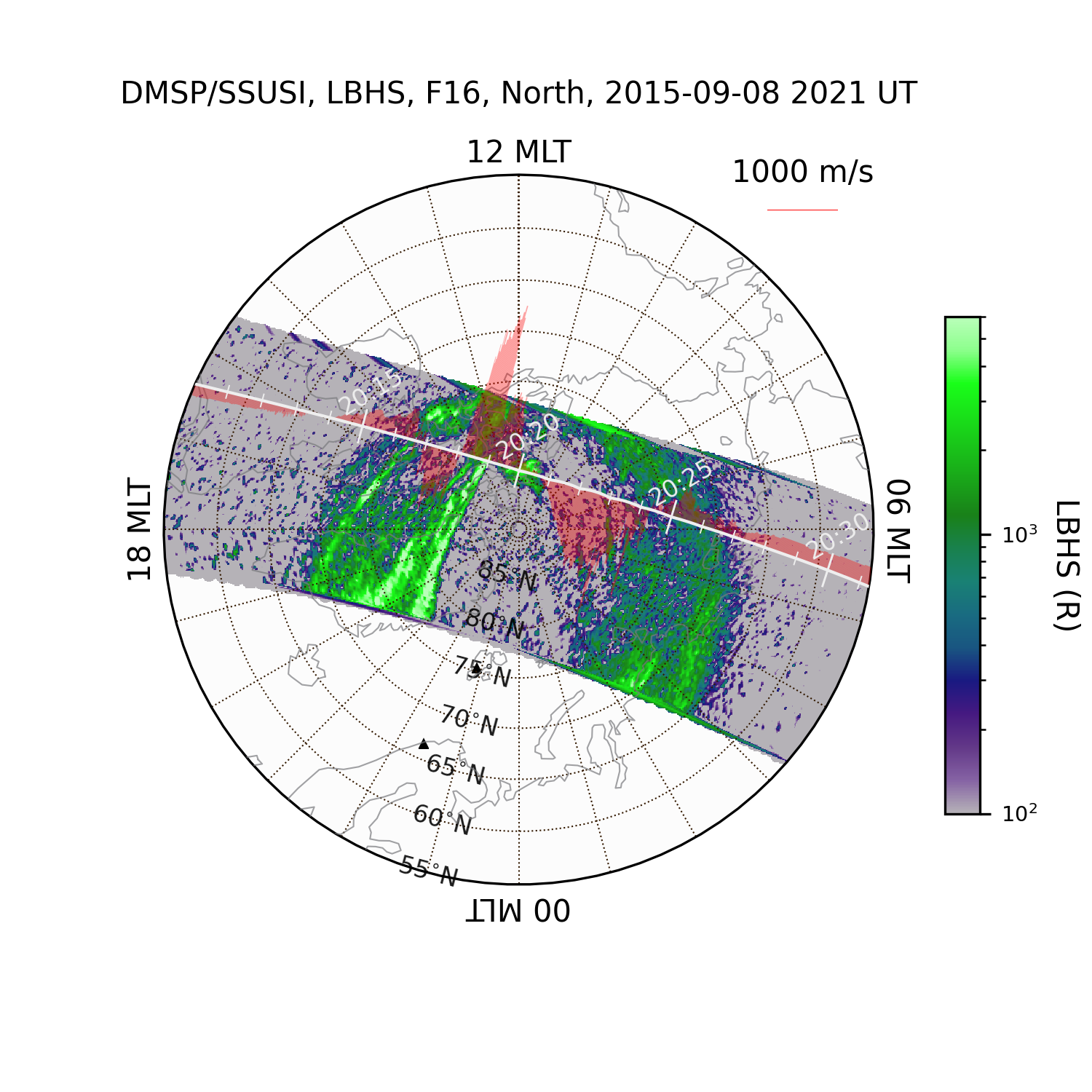 + +This is an example showing the HiLDA aurora in the dayside polar cap region +(see also [DMSP observations of the HiLDA aurora (Cai et al., JGR, 2021)](https://agupubs.onlinelibrary.wiley.com/doi/10.1029/2020JA028808)). + +Other examples for the time-series plots and map projections can be found [here](https://github.com/JouleCai/geospacelab/tree/master/examples) + +## Acknowledgements and Citation +### Acknowledgements +We acknowledge all the dependencies listed above for their contributions to implement a lot of functionality in GeospaceLAB. + +### Citation +If GeospaceLAB is used for your scientific work, please mention it in the publication and cite the package: +> Cai L, Aikio A, Kullen A, Deng Y, Zhang Y, Zhang S-R, Virtanen I and Vanhamäki H (2022), GeospaceLAB: Python package +for managing and visualizing data in space physics. Front. Astron. Space Sci. 9:1023163. doi: [10.3389/fspas.2022.1023163](https://www.frontiersin.org/articles/10.3389/fspas.2022.1023163/full) + +In addition, please add the following text in the "Methods" or "Acknowledgements" section: +> This research has made use of GeospaceLAB v?.?.?, an open-source Python package to manage and visualize data in space physics. + +Please include the project logo (see the top) to acknowledge GeospaceLAB in posters or talks. + +### Co-authorship +GeospaceLAB aims to help users to manage and visualize multiple kinds of data in space physics in a convenient way. We welcome collaboration to support your research work. If the functionality of GeospaceLAB plays a critical role in a research paper, the co-authorship is expected to be offered to one or more developers. + + +## Notes +- The current version is a pre-released version. Many features will be added soon. + + + + +%package -n python3-geospacelab +Summary: Collect, manage, and visualize geospace data. +Provides: python-geospacelab +BuildRequires: python3-devel +BuildRequires: python3-setuptools +BuildRequires: python3-pip +%description -n python3-geospacelab +<p align="center"> + <img width="500" src="https://github.com/JouleCai/geospacelab/blob/master/docs/images/logo_v1_landscape_accent_colors.png"> +</p> + +# GeospaceLAB (geospacelab) +[](https://opensource.org/licenses/BSD-3-Clause) +[](https://www.python.org/) +[](https://zenodo.org/badge/latestdoi/347315860) +[](https://pepy.tech/project/geospacelab) + +[](https://pypi.python.org/pypi/geospacelab/) + + +GeospaceLAB provides a framework of data access, analysis, and visualization for the researchers in space physics and space weather. The documentation can be found +on [readthedocs.io](https://geospacelab.readthedocs.io/en/latest/). + +## Features +- Class-based data manager, including + - __DataHub__: the core module (top-level class) to manage data from multiple sources, + - __Dataset__: the middle-level class to download, load, and process data from a data source, + - __Variable__: the base-level class to store the data array of a variable with various attributes, including its + error, name, label, unit, group, and dependencies. +- Extendable + - Provide a standard procedure from downloading, loading, and post-processing the data. + - Easy to extend for a data source which has not been supported in the package. + - Flexible to add functions for post-processing. +- Visualization + - Time series plots with + - automatically adjustable time ticks and tick labels. + - dynamical panels (flexible to add or remove panels). + - automatically detect the time gaps. + - useful marking tools (vertical line crossing panels, shadings, top bars, etc, see Example 2 in +[Usage](https://github.com/JouleCai/geospacelab#usage)) + - Map projection + - Polar views with + - coastlines in either GEO or AACGM (APEX) coordinate system. + - mapping in either fixed lon/mlon mode or in fixed LST/MLT mode. + - Support 1-D or 2-D plots with + - satellite tracks (time ticks and labels) + - nadir colored 1-D plots + - gridded surface plots +- Space coordinate system transformation + - Unified interface for cs transformations. +- Toolboxes for data analysis + - Basic toolboxes for numpy array, datetime, logging, python dict, list, and class. + +## Built-in data sources: +| Data Source | Variables | File Format | Downloadable | Express | Status | +|-----------------------------|------------------------------------|-----------------------|---------------|-----------------|--------| +| CDAWeb/OMNI | Solar wind and IMF |*cdf* | *True* | __OMNIDashboard__ | stable | +| Madrigal/EISCAT | Ionospheric Ne, Te, Ti, ... | *EISCAT-hdf5*, *Madrigal-hdf5* | *True* | __EISCATDashboard__ | stable | +| Madrigal/GNSS/TECMAP | Ionospheric GPS TEC map | *hdf5* | *True* | - | beta | +| Madrigal/DMSP/s1 | DMSP SSM, SSIES, etc | *hdf5* | *True* | __DMSPTSDashboard__ | stable | +| Madrigal/DMSP/s4 | DMSP SSIES | *hdf5* | *True* | __DMSPTSDashboard__ | stable | +| Madrigal/DMSP/e | DMSP SSJ | *hdf5* | *True* | __DMSPTSDashboard__ | stable | +| Madrigal/Millstone Hill ISR | Millstone Hill ISR | *hdf5* | *True* | __MillstoneHillISRDashboard__ | stable | +| JHUAPL/DMSP/SSUSI | DMSP SSUSI | *netcdf* | *True* | __DMSPSSUSIDashboard__ | stable | +| JHUAPL/AMPERE/fitted | AMPERE FAC | *netcdf* | *False* | __AMPEREDashboard__ | stable | +| SuperDARN/POTMAP | SuperDARN potential map | *ascii* | *False* | - | stable | +| WDC/Dst | Dst index | *IAGA2002-ASCII* | *True* | - | stable | +| WDC/ASYSYM | ASY/SYM indices | *IAGA2002-ASCII* | *True* | __OMNIDashboard__ | stable | +| WDC/AE | AE indices | *IAGA2002-ASCII* | *True* | __OMNIDashboard__ | stable | +| GFZ/Kp | Kp/Ap indices | *ASCII* | *True* | - | stable | +| GFZ/Hpo | Hp30 or Hp60 indices | *ASCII* | *True* | - | stable | +| GFZ/SNF107 | SN, F107 | *ASCII* | *True* | - | stable | +| ESA/SWARM/EFI_LP_HM | SWARM Ne, Te, etc. | *netcdf* | *True* | - | stable | +| ESA/SWARM/EFI_TCT02 | SWARM cross track vi | *netcdf* | *True* | - | stable | +| ESA/SWARM/AOB_FAC_2F | SWARM FAC, auroral oval boundary | *netcdf* | *True* | - | beta | +| TUDelft/SWARM/DNS_POD | Swarm $\rho_n$ (GPS derived) | *ASCII* | *True* | - | stable | +| TUDelft/SWARM/DNS_ACC | Swarm $\rho_n$ (GPS+Accelerometer) | *ASCII* | *True* | - | stable | +| TUDelft/GOCE/WIND_ACC | GOCE neutral wind | *ASCII* | *True* | - | stable | +| TUDelft/GRACE/WIND_ACC | GRACE neutral wind | *ASCII* | *True* | - | stable | +| TUDelft/GRACE/DNS_ACC | Grace $\rho_n$ | *ASCII* | *True* | - | stable | +| TUDelft/CHAMP/DNS_ACC | CHAMP $\rho_n$ | *ASCII* | *True* | - | stable | + | UTA/GITM/2DALL | GITM 2D output | *binary*, *IDL-sav* | *False* | - | beta | + | UTA/GITM/3DALL | GITM 3D output | *binary*, *IDL-sav* | *False* | - | beta | + + + +## Installation +### 1. The python distribution "*__Anaconda__*" is recommended: +The package was tested with the anaconda distribution and with **PYTHON>=3.7** under **Ubuntu 20.04** and **MacOS Big Sur**. + +With Anaconda, it may be easier to install some required dependencies listed below, e.g., cartopy, using the _conda_ command. +It's also recommended installing the package and dependencies in a virtual environment with anaconda. + +After [installing the anaconda distribution](https://docs.anaconda.com/anaconda/install/index.html), a virtual environment can be created by the code below in the terminal: + +```shell +conda create --name [YOUR_ENV_NAME] -c conda-forge python cython cartopy +``` +The package "spyder" is a widely-used python IDE. Other IDEs, like "VS Code" or "Pycharm" also work. + +> **_Note:_** The recommended IDE is Spyder. Sometimes, a *RuntimeError* can be raised +> when the __aacgmv2__ package is called in **PyCharm** or **VS Code**. +> If you meet this issue, try to compile the codes in **Spyder** several times. + +After creating the virtual environement, you need to activate the virtual environment: + +```shell +conda activate [YOUR_ENV_NAME] +``` +and then to install the package as shown below or to start the IDE **Spyder**. + +More detailed information to set the anaconda environment can be found [here](https://conda.io/projects/conda/en/latest/user-guide/tasks/manage-environments.html#), + +### 2. Installation +#### Quick install from the pre-built release (recommended): +```shell +pip install geospacelab +``` + +#### Install from [Github](https://github.com/JouleCai/geospacelab) (not recommended): +```shell +pip install git+https://github.com/JouleCai/geospacelab@master +``` + +### 2. Dependencies +The package dependencies need to be installed before or after the installation of the package. +Several dependencies will be installed automatically with the package installation, +including __toml__, __requests__, __bueatifulsoup4__, __numpy__, __scipy__, __matplotlib__, __h5py__, __netcdf4__, +__cdflib__, __madrigalweb__, __sscws__, and __aacgmv2__. + +Other dependencies will be needed if you see a *__ImportError__* or *__ModuleNotFoundError__* +displayed in the python console. Some frequently used modules and their installation methods are listed below: +- [__cartopy__](https://scitools.org.uk/cartopy/docs/latest/installing.html): Map projection for geospatial data. + - ```conda install -c conda-forge cartopy ``` +- [__apexpy__ \*](https://apexpy.readthedocs.io/en/latest/reference/Apex.html): Apex and Quasi-Dipole geomagnetic +coordinate system. + - ```pip install apexpy ``` +- [__geopack__](https://github.com/tsssss/geopack): The geopack and Tsyganenko models in Python. + - ```pip install geopack ``` + +> ([\*]()): The **_gcc_** or **_gfortran_** compilers are required before installing the package. +> - gcc: ```conda install -c conda-forge gcc``` +> - gfortran: ```conda install -c conda-forge gfortran ``` + +Please install the packages above, if needed. + +Note: The package is currently pre-released. The installation methods may be changed in the future. + + +### 4. First-time startup and basic configuration +Some basic configurations will be made with the first-time import of the package. Following the messages prompted in the python console, the first configuration is to set the root directory for storing the data. + +When the modules to access the online Madrigal database is imported, it will ask for the inputs of user's full name, email, and affiliation. + +The user's configuration can be found from the *__toml__* file below: +``` +[your_home_directory]/.geospacelab/config.toml +``` +The user can set or change the preferences in the configuration file. For example, to change the root directory for storing the data, modify or add the lines in "config.toml": +```toml +[datahub] +data_root_dir = "YOUR_ROOT_DIR" +``` +To set the Madrigal cookies, change the lines: +```toml +[datahub.madrigal] +user_fullname = "YOUR_NAME" +user_email = "YOU_EMAIL" +user_affiliation = "YOUR_AFFILIATION" +``` + +### 5. Upgrade + +If the package is installed from the pre-built release. Update the package via: +```shell +pip install geospacelab --upgrade +``` + +### 6. Uninstallation +Uninstall the package via: +```shell +pip uninstall geospacelab +``` +If you don't need the user's configuration, delete the file at **_[your_home_directory]/.geospacelab/config.toml_** + +## Usage +### Example 1: Dock a sourced dataset and get variables: +The core of the data manager is the class Datahub. A Datahub instance will be used for docking a buit-in sourced dataset, or adding a temporary or user-defined dataset. + +The "dataset" is a Dataset instance, which is used for loading and downloading +the data. + +Below is an example to load the EISCAT data from the online service. The module will download EISCAT data automatically from +[the EISCAT schedule page](https://portal.eiscat.se/schedule/) with the presetttings of loading mode "AUTO" and file type "eiscat-hdf5". + +Example 1: +```python +import datetime + +from geospacelab.datahub import DataHub + +# settings +dt_fr = datetime.datetime.strptime('20210309' + '0000', '%Y%m%d%H%M') # datetime from +dt_to = datetime.datetime.strptime('20210309' + '2359', '%Y%m%d%H%M') # datetime to +database_name = 'madrigal' # built-in sourced database name +facility_name = 'eiscat' # facility name + +site = 'UHF' # facility attributes required, check from the eiscat schedule page +antenna = 'UHF' +modulation = 'ant' + +# create a datahub instance +dh = DataHub(dt_fr, dt_to) +# dock the first dataset (dataset index starts from 0) +ds_isr = dh.dock(datasource_contents=[database_name, 'isr', facility_name], + site=site, antenna=antenna, modulation=modulation, data_file_type='eiscat-hdf5') +# load data +ds_isr.load_data() +# assign a variable from its own dataset to the datahub +n_e = dh.assign_variable('n_e') +T_i = dh.assign_variable('T_i') + +# get the variables which have been assigned in the datahub +n_e = dh.get_variable('n_e') +T_i = dh.get_variable('T_i') +# if the variable is not assigned in the datahub, but exists in the its own dataset: +comp_O_p = dh.get_variable('comp_O_p', dataset=ds_isr) # O+ ratio +# above line is equivalent to +comp_O_p = dh.datasets[0]['comp_O_p'] + +# The variables, e.g., n_e and T_i, are the class Variable's instances, +# which stores the variable values, errors, and many other attributes, e.g., name, label, unit, depends, .... +# To get the value of the variable, use variable_isntance.value, e.g., +print(n_e.value) # return the variable's value, type: numpy.ndarray, axis 0 is always along the time, check n_e.depends.items{} +print(n_e.error) + +``` + +### Example 2: EISCAT quicklook plot +The EISCAT quicklook plot shows the GUISDAP analysed results in the same format as the online EISCAT quicklook plot. +The figure layout and quality are improved. In addition, several marking tools like vertical lines, shadings, top bars can be +added in the plot. See the example script and figure below: + +In "example2.py" +```python +import datetime +import geospacelab.express.eiscat_dashboard as eiscat + +dt_fr = datetime.datetime.strptime('20201209' + '1800', '%Y%m%d%H%M') +dt_to = datetime.datetime.strptime('20201210' + '0600', '%Y%m%d%H%M') + +site = 'UHF' +antenna = 'UHF' +modulation = '60' +load_mode = 'AUTO' +dashboard = eiscat.EISCATDashboard( + dt_fr, dt_to, site=site, antenna=antenna, modulation=modulation, load_mode='AUTO' +) +dashboard.quicklook() + +# dashboard.save_figure() # comment this if you need to run the following codes +# dashboard.show() # comment this if you need to run the following codes. + +""" +As the dashboard class (EISCATDashboard) is a inheritance of the classes Datahub and TSDashboard. +The variables can be retrieved in the same ways as shown in Example 1. +""" +n_e = dashboard.assign_variable('n_e') +print(n_e.value) +print(n_e.error) + +""" +Several marking tools (vertical lines, shadings, and top bars) can be added as the overlays +on the top of the quicklook plot. +""" +# add vertical line +dt_fr_2 = datetime.datetime.strptime('20201209' + '2030', "%Y%m%d%H%M") +dt_to_2 = datetime.datetime.strptime('20201210' + '0130', "%Y%m%d%H%M") +dashboard.add_vertical_line(dt_fr_2, bottom_extend=0, top_extend=0.02, label='Line 1', label_position='top') +# add shading +dashboard.add_shading(dt_fr_2, dt_to_2, bottom_extend=0, top_extend=0.02, label='Shading 1', label_position='top') +# add top bar +dt_fr_3 = datetime.datetime.strptime('20201210' + '0130', "%Y%m%d%H%M") +dt_to_3 = datetime.datetime.strptime('20201210' + '0430', "%Y%m%d%H%M") +dashboard.add_top_bar(dt_fr_3, dt_to_3, bottom=0., top=0.02, label='Top bar 1') + +# save figure +dashboard.save_figure() +# show on screen +dashboard.show() +``` +Output: +>  + +### Example 3: OMNI data and geomagnetic indices (WDC + GFZ): + +In "example3.py" + +```python +import datetime +import geospacelab.express.omni_dashboard as omni + +dt_fr = datetime.datetime.strptime('20160314' + '0600', '%Y%m%d%H%M') +dt_to = datetime.datetime.strptime('20160320' + '0600', '%Y%m%d%H%M') + +omni_type = 'OMNI2' +omni_res = '1min' +load_mode = 'AUTO' +dashboard = omni.OMNIDashboard( + dt_fr, dt_to, omni_type=omni_type, omni_res=omni_res, load_mode=load_mode +) +dashboard.quicklook() + +# data can be retrieved in the same way as in Example 1: +dashboard.list_assigned_variables() +B_x_gsm = dashboard.get_variable('B_x_GSM', dataset_index=0) +# save figure +dashboard.save_figure() +# show on screen +dashboard.show() +``` +Output: +>  + +### Example 4: Mapping geospatial data in the polar map. +```python +import datetime +import matplotlib.pyplot as plt + +import geospacelab.visualization.mpl.geomap.geodashboards as geomap + +dt_fr = datetime.datetime(2015, 9, 8, 8) +dt_to = datetime.datetime(2015, 9, 8, 23, 59) +time1 = datetime.datetime(2015, 9, 8, 20, 21) +pole = 'N' +sat_id = 'f16' +band = 'LBHS' + +# Create a geodashboard object +dashboard = geomap.GeoDashboard(dt_fr=dt_fr, dt_to=dt_to, figure_config={'figsize': (5, 5)}) + +# If the orbit_id is specified, only one file will be downloaded. This option saves the downloading time. +# dashboard.dock(datasource_contents=['jhuapl', 'dmsp', 'ssusi', 'edraur'], pole='N', sat_id='f17', orbit_id='46863') +# If not specified, the data during the whole day will be downloaded. +dashboard.dock(datasource_contents=['jhuapl', 'dmsp', 'ssusi', 'edraur'], pole=pole, sat_id=sat_id, orbit_id=None) +ds_s1 = dashboard.dock( + datasource_contents=['madrigal', 'satellites', 'dmsp', 's1'], + dt_fr=time1 - datetime.timedelta(minutes=45), + dt_to=time1 + datetime.timedelta(minutes=45), + sat_id=sat_id) + +dashboard.set_layout(1, 1) + +# Get the variables: LBHS emission intensiy, corresponding times and locations +lbhs = dashboard.assign_variable('GRID_AUR_' + band, dataset_index=0) +dts = dashboard.assign_variable('DATETIME', dataset_index=0).value.flatten() +mlat = dashboard.assign_variable('GRID_MLAT', dataset_index=0).value +mlon = dashboard.assign_variable('GRID_MLON', dataset_index=0).value +mlt = dashboard.assign_variable(('GRID_MLT'), dataset_index=0).value + +# Search the index for the time to plot, used as an input to the following polar map +ind_t = dashboard.datasets[0].get_time_ind(ut=time1) +lbhs_ = lbhs.value[ind_t] +mlat_ = mlat[ind_t] +mlon_ = mlon[ind_t] +mlt_ = mlt[ind_t] +# Add a polar map panel to the dashboard. Currently the style is the fixed MLT at mlt_c=0. See the keywords below: +panel1 = dashboard.add_polar_map(row_ind=0, col_ind=0, style='mlt-fixed', cs='AACGM', mlt_c=0., pole=pole, ut=time1, boundary_lat=65., mirror_south=True) + +# Some settings for plotting. +pcolormesh_config = lbhs.visual.plot_config.pcolormesh +# Overlay the SSUSI image in the map. +ipm = panel1.overlay_pcolormesh(data=lbhs_, coords={'lat': mlat_, 'lon': mlon_, 'mlt': mlt_}, cs='AACGM', + regridding=True, **pcolormesh_config) +# Add a color bar +panel1.add_colorbar(ipm, c_label=band + " (R)", c_scale=pcolormesh_config['c_scale'], left=1.1, bottom=0.1, + width=0.05, height=0.7) + +# Overlay the gridlines +panel1.overlay_gridlines(lat_res=5, lon_label_separator=5) + +# Overlay the coastlines in the AACGM coordinate +panel1.overlay_coastlines() + +# Overlay cross-track velocity along satellite trajectory +sc_dt = ds_s1['SC_DATETIME'].value.flatten() +sc_lat = ds_s1['SC_GEO_LAT'].value.flatten() +sc_lon = ds_s1['SC_GEO_LON'].value.flatten() +sc_alt = ds_s1['SC_GEO_ALT'].value.flatten() +sc_coords = {'lat': sc_lat, 'lon': sc_lon, 'height': sc_alt} + +v_H = ds_s1['v_i_H'].value.flatten() +panel1.overlay_cross_track_vector(vector=v_H, unit_vector=1000, alpha=0.5, color='r', sc_coords=sc_coords, sc_ut=sc_dt, cs='GEOC') +# Overlay the satellite trajectory with ticks +panel1.overlay_sc_trajectory(sc_ut=sc_dt, sc_coords=sc_coords, cs='GEOC') + +# Add the title and save the figure +polestr = 'North' if pole == 'N' else 'South' +panel1.add_title(title='DMSP/SSUSI, ' + band + ', ' + sat_id.upper() + ', ' + polestr + ', ' + time1.strftime('%Y-%m-%d %H%M UT')) +plt.savefig('DMSP_SSUSI_' + time1.strftime('%Y%m%d-%H%M') + '_' + band + '_' + sat_id.upper() + '_' + pole, dpi=300) + +# show the figure +plt.show() +``` +Output: +>  + +This is an example showing the HiLDA aurora in the dayside polar cap region +(see also [DMSP observations of the HiLDA aurora (Cai et al., JGR, 2021)](https://agupubs.onlinelibrary.wiley.com/doi/10.1029/2020JA028808)). + +Other examples for the time-series plots and map projections can be found [here](https://github.com/JouleCai/geospacelab/tree/master/examples) + +## Acknowledgements and Citation +### Acknowledgements +We acknowledge all the dependencies listed above for their contributions to implement a lot of functionality in GeospaceLAB. + +### Citation +If GeospaceLAB is used for your scientific work, please mention it in the publication and cite the package: +> Cai L, Aikio A, Kullen A, Deng Y, Zhang Y, Zhang S-R, Virtanen I and Vanhamäki H (2022), GeospaceLAB: Python package +for managing and visualizing data in space physics. Front. Astron. Space Sci. 9:1023163. doi: [10.3389/fspas.2022.1023163](https://www.frontiersin.org/articles/10.3389/fspas.2022.1023163/full) + +In addition, please add the following text in the "Methods" or "Acknowledgements" section: +> This research has made use of GeospaceLAB v?.?.?, an open-source Python package to manage and visualize data in space physics. + +Please include the project logo (see the top) to acknowledge GeospaceLAB in posters or talks. + +### Co-authorship +GeospaceLAB aims to help users to manage and visualize multiple kinds of data in space physics in a convenient way. We welcome collaboration to support your research work. If the functionality of GeospaceLAB plays a critical role in a research paper, the co-authorship is expected to be offered to one or more developers. + + +## Notes +- The current version is a pre-released version. Many features will be added soon. + + + + +%package help +Summary: Development documents and examples for geospacelab +Provides: python3-geospacelab-doc +%description help +<p align="center"> + <img width="500" src="https://github.com/JouleCai/geospacelab/blob/master/docs/images/logo_v1_landscape_accent_colors.png"> +</p> + +# GeospaceLAB (geospacelab) +[](https://opensource.org/licenses/BSD-3-Clause) +[](https://www.python.org/) +[](https://zenodo.org/badge/latestdoi/347315860) +[](https://pepy.tech/project/geospacelab) + +[](https://pypi.python.org/pypi/geospacelab/) + + +GeospaceLAB provides a framework of data access, analysis, and visualization for the researchers in space physics and space weather. The documentation can be found +on [readthedocs.io](https://geospacelab.readthedocs.io/en/latest/). + +## Features +- Class-based data manager, including + - __DataHub__: the core module (top-level class) to manage data from multiple sources, + - __Dataset__: the middle-level class to download, load, and process data from a data source, + - __Variable__: the base-level class to store the data array of a variable with various attributes, including its + error, name, label, unit, group, and dependencies. +- Extendable + - Provide a standard procedure from downloading, loading, and post-processing the data. + - Easy to extend for a data source which has not been supported in the package. + - Flexible to add functions for post-processing. +- Visualization + - Time series plots with + - automatically adjustable time ticks and tick labels. + - dynamical panels (flexible to add or remove panels). + - automatically detect the time gaps. + - useful marking tools (vertical line crossing panels, shadings, top bars, etc, see Example 2 in +[Usage](https://github.com/JouleCai/geospacelab#usage)) + - Map projection + - Polar views with + - coastlines in either GEO or AACGM (APEX) coordinate system. + - mapping in either fixed lon/mlon mode or in fixed LST/MLT mode. + - Support 1-D or 2-D plots with + - satellite tracks (time ticks and labels) + - nadir colored 1-D plots + - gridded surface plots +- Space coordinate system transformation + - Unified interface for cs transformations. +- Toolboxes for data analysis + - Basic toolboxes for numpy array, datetime, logging, python dict, list, and class. + +## Built-in data sources: +| Data Source | Variables | File Format | Downloadable | Express | Status | +|-----------------------------|------------------------------------|-----------------------|---------------|-----------------|--------| +| CDAWeb/OMNI | Solar wind and IMF |*cdf* | *True* | __OMNIDashboard__ | stable | +| Madrigal/EISCAT | Ionospheric Ne, Te, Ti, ... | *EISCAT-hdf5*, *Madrigal-hdf5* | *True* | __EISCATDashboard__ | stable | +| Madrigal/GNSS/TECMAP | Ionospheric GPS TEC map | *hdf5* | *True* | - | beta | +| Madrigal/DMSP/s1 | DMSP SSM, SSIES, etc | *hdf5* | *True* | __DMSPTSDashboard__ | stable | +| Madrigal/DMSP/s4 | DMSP SSIES | *hdf5* | *True* | __DMSPTSDashboard__ | stable | +| Madrigal/DMSP/e | DMSP SSJ | *hdf5* | *True* | __DMSPTSDashboard__ | stable | +| Madrigal/Millstone Hill ISR | Millstone Hill ISR | *hdf5* | *True* | __MillstoneHillISRDashboard__ | stable | +| JHUAPL/DMSP/SSUSI | DMSP SSUSI | *netcdf* | *True* | __DMSPSSUSIDashboard__ | stable | +| JHUAPL/AMPERE/fitted | AMPERE FAC | *netcdf* | *False* | __AMPEREDashboard__ | stable | +| SuperDARN/POTMAP | SuperDARN potential map | *ascii* | *False* | - | stable | +| WDC/Dst | Dst index | *IAGA2002-ASCII* | *True* | - | stable | +| WDC/ASYSYM | ASY/SYM indices | *IAGA2002-ASCII* | *True* | __OMNIDashboard__ | stable | +| WDC/AE | AE indices | *IAGA2002-ASCII* | *True* | __OMNIDashboard__ | stable | +| GFZ/Kp | Kp/Ap indices | *ASCII* | *True* | - | stable | +| GFZ/Hpo | Hp30 or Hp60 indices | *ASCII* | *True* | - | stable | +| GFZ/SNF107 | SN, F107 | *ASCII* | *True* | - | stable | +| ESA/SWARM/EFI_LP_HM | SWARM Ne, Te, etc. | *netcdf* | *True* | - | stable | +| ESA/SWARM/EFI_TCT02 | SWARM cross track vi | *netcdf* | *True* | - | stable | +| ESA/SWARM/AOB_FAC_2F | SWARM FAC, auroral oval boundary | *netcdf* | *True* | - | beta | +| TUDelft/SWARM/DNS_POD | Swarm $\rho_n$ (GPS derived) | *ASCII* | *True* | - | stable | +| TUDelft/SWARM/DNS_ACC | Swarm $\rho_n$ (GPS+Accelerometer) | *ASCII* | *True* | - | stable | +| TUDelft/GOCE/WIND_ACC | GOCE neutral wind | *ASCII* | *True* | - | stable | +| TUDelft/GRACE/WIND_ACC | GRACE neutral wind | *ASCII* | *True* | - | stable | +| TUDelft/GRACE/DNS_ACC | Grace $\rho_n$ | *ASCII* | *True* | - | stable | +| TUDelft/CHAMP/DNS_ACC | CHAMP $\rho_n$ | *ASCII* | *True* | - | stable | + | UTA/GITM/2DALL | GITM 2D output | *binary*, *IDL-sav* | *False* | - | beta | + | UTA/GITM/3DALL | GITM 3D output | *binary*, *IDL-sav* | *False* | - | beta | + + + +## Installation +### 1. The python distribution "*__Anaconda__*" is recommended: +The package was tested with the anaconda distribution and with **PYTHON>=3.7** under **Ubuntu 20.04** and **MacOS Big Sur**. + +With Anaconda, it may be easier to install some required dependencies listed below, e.g., cartopy, using the _conda_ command. +It's also recommended installing the package and dependencies in a virtual environment with anaconda. + +After [installing the anaconda distribution](https://docs.anaconda.com/anaconda/install/index.html), a virtual environment can be created by the code below in the terminal: + +```shell +conda create --name [YOUR_ENV_NAME] -c conda-forge python cython cartopy +``` +The package "spyder" is a widely-used python IDE. Other IDEs, like "VS Code" or "Pycharm" also work. + +> **_Note:_** The recommended IDE is Spyder. Sometimes, a *RuntimeError* can be raised +> when the __aacgmv2__ package is called in **PyCharm** or **VS Code**. +> If you meet this issue, try to compile the codes in **Spyder** several times. + +After creating the virtual environement, you need to activate the virtual environment: + +```shell +conda activate [YOUR_ENV_NAME] +``` +and then to install the package as shown below or to start the IDE **Spyder**. + +More detailed information to set the anaconda environment can be found [here](https://conda.io/projects/conda/en/latest/user-guide/tasks/manage-environments.html#), + +### 2. Installation +#### Quick install from the pre-built release (recommended): +```shell +pip install geospacelab +``` + +#### Install from [Github](https://github.com/JouleCai/geospacelab) (not recommended): +```shell +pip install git+https://github.com/JouleCai/geospacelab@master +``` + +### 2. Dependencies +The package dependencies need to be installed before or after the installation of the package. +Several dependencies will be installed automatically with the package installation, +including __toml__, __requests__, __bueatifulsoup4__, __numpy__, __scipy__, __matplotlib__, __h5py__, __netcdf4__, +__cdflib__, __madrigalweb__, __sscws__, and __aacgmv2__. + +Other dependencies will be needed if you see a *__ImportError__* or *__ModuleNotFoundError__* +displayed in the python console. Some frequently used modules and their installation methods are listed below: +- [__cartopy__](https://scitools.org.uk/cartopy/docs/latest/installing.html): Map projection for geospatial data. + - ```conda install -c conda-forge cartopy ``` +- [__apexpy__ \*](https://apexpy.readthedocs.io/en/latest/reference/Apex.html): Apex and Quasi-Dipole geomagnetic +coordinate system. + - ```pip install apexpy ``` +- [__geopack__](https://github.com/tsssss/geopack): The geopack and Tsyganenko models in Python. + - ```pip install geopack ``` + +> ([\*]()): The **_gcc_** or **_gfortran_** compilers are required before installing the package. +> - gcc: ```conda install -c conda-forge gcc``` +> - gfortran: ```conda install -c conda-forge gfortran ``` + +Please install the packages above, if needed. + +Note: The package is currently pre-released. The installation methods may be changed in the future. + + +### 4. First-time startup and basic configuration +Some basic configurations will be made with the first-time import of the package. Following the messages prompted in the python console, the first configuration is to set the root directory for storing the data. + +When the modules to access the online Madrigal database is imported, it will ask for the inputs of user's full name, email, and affiliation. + +The user's configuration can be found from the *__toml__* file below: +``` +[your_home_directory]/.geospacelab/config.toml +``` +The user can set or change the preferences in the configuration file. For example, to change the root directory for storing the data, modify or add the lines in "config.toml": +```toml +[datahub] +data_root_dir = "YOUR_ROOT_DIR" +``` +To set the Madrigal cookies, change the lines: +```toml +[datahub.madrigal] +user_fullname = "YOUR_NAME" +user_email = "YOU_EMAIL" +user_affiliation = "YOUR_AFFILIATION" +``` + +### 5. Upgrade + +If the package is installed from the pre-built release. Update the package via: +```shell +pip install geospacelab --upgrade +``` + +### 6. Uninstallation +Uninstall the package via: +```shell +pip uninstall geospacelab +``` +If you don't need the user's configuration, delete the file at **_[your_home_directory]/.geospacelab/config.toml_** + +## Usage +### Example 1: Dock a sourced dataset and get variables: +The core of the data manager is the class Datahub. A Datahub instance will be used for docking a buit-in sourced dataset, or adding a temporary or user-defined dataset. + +The "dataset" is a Dataset instance, which is used for loading and downloading +the data. + +Below is an example to load the EISCAT data from the online service. The module will download EISCAT data automatically from +[the EISCAT schedule page](https://portal.eiscat.se/schedule/) with the presetttings of loading mode "AUTO" and file type "eiscat-hdf5". + +Example 1: +```python +import datetime + +from geospacelab.datahub import DataHub + +# settings +dt_fr = datetime.datetime.strptime('20210309' + '0000', '%Y%m%d%H%M') # datetime from +dt_to = datetime.datetime.strptime('20210309' + '2359', '%Y%m%d%H%M') # datetime to +database_name = 'madrigal' # built-in sourced database name +facility_name = 'eiscat' # facility name + +site = 'UHF' # facility attributes required, check from the eiscat schedule page +antenna = 'UHF' +modulation = 'ant' + +# create a datahub instance +dh = DataHub(dt_fr, dt_to) +# dock the first dataset (dataset index starts from 0) +ds_isr = dh.dock(datasource_contents=[database_name, 'isr', facility_name], + site=site, antenna=antenna, modulation=modulation, data_file_type='eiscat-hdf5') +# load data +ds_isr.load_data() +# assign a variable from its own dataset to the datahub +n_e = dh.assign_variable('n_e') +T_i = dh.assign_variable('T_i') + +# get the variables which have been assigned in the datahub +n_e = dh.get_variable('n_e') +T_i = dh.get_variable('T_i') +# if the variable is not assigned in the datahub, but exists in the its own dataset: +comp_O_p = dh.get_variable('comp_O_p', dataset=ds_isr) # O+ ratio +# above line is equivalent to +comp_O_p = dh.datasets[0]['comp_O_p'] + +# The variables, e.g., n_e and T_i, are the class Variable's instances, +# which stores the variable values, errors, and many other attributes, e.g., name, label, unit, depends, .... +# To get the value of the variable, use variable_isntance.value, e.g., +print(n_e.value) # return the variable's value, type: numpy.ndarray, axis 0 is always along the time, check n_e.depends.items{} +print(n_e.error) + +``` + +### Example 2: EISCAT quicklook plot +The EISCAT quicklook plot shows the GUISDAP analysed results in the same format as the online EISCAT quicklook plot. +The figure layout and quality are improved. In addition, several marking tools like vertical lines, shadings, top bars can be +added in the plot. See the example script and figure below: + +In "example2.py" +```python +import datetime +import geospacelab.express.eiscat_dashboard as eiscat + +dt_fr = datetime.datetime.strptime('20201209' + '1800', '%Y%m%d%H%M') +dt_to = datetime.datetime.strptime('20201210' + '0600', '%Y%m%d%H%M') + +site = 'UHF' +antenna = 'UHF' +modulation = '60' +load_mode = 'AUTO' +dashboard = eiscat.EISCATDashboard( + dt_fr, dt_to, site=site, antenna=antenna, modulation=modulation, load_mode='AUTO' +) +dashboard.quicklook() + +# dashboard.save_figure() # comment this if you need to run the following codes +# dashboard.show() # comment this if you need to run the following codes. + +""" +As the dashboard class (EISCATDashboard) is a inheritance of the classes Datahub and TSDashboard. +The variables can be retrieved in the same ways as shown in Example 1. +""" +n_e = dashboard.assign_variable('n_e') +print(n_e.value) +print(n_e.error) + +""" +Several marking tools (vertical lines, shadings, and top bars) can be added as the overlays +on the top of the quicklook plot. +""" +# add vertical line +dt_fr_2 = datetime.datetime.strptime('20201209' + '2030', "%Y%m%d%H%M") +dt_to_2 = datetime.datetime.strptime('20201210' + '0130', "%Y%m%d%H%M") +dashboard.add_vertical_line(dt_fr_2, bottom_extend=0, top_extend=0.02, label='Line 1', label_position='top') +# add shading +dashboard.add_shading(dt_fr_2, dt_to_2, bottom_extend=0, top_extend=0.02, label='Shading 1', label_position='top') +# add top bar +dt_fr_3 = datetime.datetime.strptime('20201210' + '0130', "%Y%m%d%H%M") +dt_to_3 = datetime.datetime.strptime('20201210' + '0430', "%Y%m%d%H%M") +dashboard.add_top_bar(dt_fr_3, dt_to_3, bottom=0., top=0.02, label='Top bar 1') + +# save figure +dashboard.save_figure() +# show on screen +dashboard.show() +``` +Output: +>  + +### Example 3: OMNI data and geomagnetic indices (WDC + GFZ): + +In "example3.py" + +```python +import datetime +import geospacelab.express.omni_dashboard as omni + +dt_fr = datetime.datetime.strptime('20160314' + '0600', '%Y%m%d%H%M') +dt_to = datetime.datetime.strptime('20160320' + '0600', '%Y%m%d%H%M') + +omni_type = 'OMNI2' +omni_res = '1min' +load_mode = 'AUTO' +dashboard = omni.OMNIDashboard( + dt_fr, dt_to, omni_type=omni_type, omni_res=omni_res, load_mode=load_mode +) +dashboard.quicklook() + +# data can be retrieved in the same way as in Example 1: +dashboard.list_assigned_variables() +B_x_gsm = dashboard.get_variable('B_x_GSM', dataset_index=0) +# save figure +dashboard.save_figure() +# show on screen +dashboard.show() +``` +Output: +>  + +### Example 4: Mapping geospatial data in the polar map. +```python +import datetime +import matplotlib.pyplot as plt + +import geospacelab.visualization.mpl.geomap.geodashboards as geomap + +dt_fr = datetime.datetime(2015, 9, 8, 8) +dt_to = datetime.datetime(2015, 9, 8, 23, 59) +time1 = datetime.datetime(2015, 9, 8, 20, 21) +pole = 'N' +sat_id = 'f16' +band = 'LBHS' + +# Create a geodashboard object +dashboard = geomap.GeoDashboard(dt_fr=dt_fr, dt_to=dt_to, figure_config={'figsize': (5, 5)}) + +# If the orbit_id is specified, only one file will be downloaded. This option saves the downloading time. +# dashboard.dock(datasource_contents=['jhuapl', 'dmsp', 'ssusi', 'edraur'], pole='N', sat_id='f17', orbit_id='46863') +# If not specified, the data during the whole day will be downloaded. +dashboard.dock(datasource_contents=['jhuapl', 'dmsp', 'ssusi', 'edraur'], pole=pole, sat_id=sat_id, orbit_id=None) +ds_s1 = dashboard.dock( + datasource_contents=['madrigal', 'satellites', 'dmsp', 's1'], + dt_fr=time1 - datetime.timedelta(minutes=45), + dt_to=time1 + datetime.timedelta(minutes=45), + sat_id=sat_id) + +dashboard.set_layout(1, 1) + +# Get the variables: LBHS emission intensiy, corresponding times and locations +lbhs = dashboard.assign_variable('GRID_AUR_' + band, dataset_index=0) +dts = dashboard.assign_variable('DATETIME', dataset_index=0).value.flatten() +mlat = dashboard.assign_variable('GRID_MLAT', dataset_index=0).value +mlon = dashboard.assign_variable('GRID_MLON', dataset_index=0).value +mlt = dashboard.assign_variable(('GRID_MLT'), dataset_index=0).value + +# Search the index for the time to plot, used as an input to the following polar map +ind_t = dashboard.datasets[0].get_time_ind(ut=time1) +lbhs_ = lbhs.value[ind_t] +mlat_ = mlat[ind_t] +mlon_ = mlon[ind_t] +mlt_ = mlt[ind_t] +# Add a polar map panel to the dashboard. Currently the style is the fixed MLT at mlt_c=0. See the keywords below: +panel1 = dashboard.add_polar_map(row_ind=0, col_ind=0, style='mlt-fixed', cs='AACGM', mlt_c=0., pole=pole, ut=time1, boundary_lat=65., mirror_south=True) + +# Some settings for plotting. +pcolormesh_config = lbhs.visual.plot_config.pcolormesh +# Overlay the SSUSI image in the map. +ipm = panel1.overlay_pcolormesh(data=lbhs_, coords={'lat': mlat_, 'lon': mlon_, 'mlt': mlt_}, cs='AACGM', + regridding=True, **pcolormesh_config) +# Add a color bar +panel1.add_colorbar(ipm, c_label=band + " (R)", c_scale=pcolormesh_config['c_scale'], left=1.1, bottom=0.1, + width=0.05, height=0.7) + +# Overlay the gridlines +panel1.overlay_gridlines(lat_res=5, lon_label_separator=5) + +# Overlay the coastlines in the AACGM coordinate +panel1.overlay_coastlines() + +# Overlay cross-track velocity along satellite trajectory +sc_dt = ds_s1['SC_DATETIME'].value.flatten() +sc_lat = ds_s1['SC_GEO_LAT'].value.flatten() +sc_lon = ds_s1['SC_GEO_LON'].value.flatten() +sc_alt = ds_s1['SC_GEO_ALT'].value.flatten() +sc_coords = {'lat': sc_lat, 'lon': sc_lon, 'height': sc_alt} + +v_H = ds_s1['v_i_H'].value.flatten() +panel1.overlay_cross_track_vector(vector=v_H, unit_vector=1000, alpha=0.5, color='r', sc_coords=sc_coords, sc_ut=sc_dt, cs='GEOC') +# Overlay the satellite trajectory with ticks +panel1.overlay_sc_trajectory(sc_ut=sc_dt, sc_coords=sc_coords, cs='GEOC') + +# Add the title and save the figure +polestr = 'North' if pole == 'N' else 'South' +panel1.add_title(title='DMSP/SSUSI, ' + band + ', ' + sat_id.upper() + ', ' + polestr + ', ' + time1.strftime('%Y-%m-%d %H%M UT')) +plt.savefig('DMSP_SSUSI_' + time1.strftime('%Y%m%d-%H%M') + '_' + band + '_' + sat_id.upper() + '_' + pole, dpi=300) + +# show the figure +plt.show() +``` +Output: +>  + +This is an example showing the HiLDA aurora in the dayside polar cap region +(see also [DMSP observations of the HiLDA aurora (Cai et al., JGR, 2021)](https://agupubs.onlinelibrary.wiley.com/doi/10.1029/2020JA028808)). + +Other examples for the time-series plots and map projections can be found [here](https://github.com/JouleCai/geospacelab/tree/master/examples) + +## Acknowledgements and Citation +### Acknowledgements +We acknowledge all the dependencies listed above for their contributions to implement a lot of functionality in GeospaceLAB. + +### Citation +If GeospaceLAB is used for your scientific work, please mention it in the publication and cite the package: +> Cai L, Aikio A, Kullen A, Deng Y, Zhang Y, Zhang S-R, Virtanen I and Vanhamäki H (2022), GeospaceLAB: Python package +for managing and visualizing data in space physics. Front. Astron. Space Sci. 9:1023163. doi: [10.3389/fspas.2022.1023163](https://www.frontiersin.org/articles/10.3389/fspas.2022.1023163/full) + +In addition, please add the following text in the "Methods" or "Acknowledgements" section: +> This research has made use of GeospaceLAB v?.?.?, an open-source Python package to manage and visualize data in space physics. + +Please include the project logo (see the top) to acknowledge GeospaceLAB in posters or talks. + +### Co-authorship +GeospaceLAB aims to help users to manage and visualize multiple kinds of data in space physics in a convenient way. We welcome collaboration to support your research work. If the functionality of GeospaceLAB plays a critical role in a research paper, the co-authorship is expected to be offered to one or more developers. + + +## Notes +- The current version is a pre-released version. Many features will be added soon. + + + + +%prep +%autosetup -n geospacelab-0.6.1 + +%build +%py3_build + +%install +%py3_install +install -d -m755 %{buildroot}/%{_pkgdocdir} +if [ -d doc ]; then cp -arf doc %{buildroot}/%{_pkgdocdir}; fi +if [ -d docs ]; then cp -arf docs %{buildroot}/%{_pkgdocdir}; fi +if [ -d example ]; then cp -arf example %{buildroot}/%{_pkgdocdir}; fi +if [ -d examples ]; then cp -arf examples %{buildroot}/%{_pkgdocdir}; fi +pushd %{buildroot} +if [ -d usr/lib ]; then + find usr/lib -type f -printf "/%h/%f\n" >> filelist.lst +fi +if [ -d usr/lib64 ]; then + find usr/lib64 -type f -printf "/%h/%f\n" >> filelist.lst +fi +if [ -d usr/bin ]; then + find usr/bin -type f -printf "/%h/%f\n" >> filelist.lst +fi +if [ -d usr/sbin ]; then + find usr/sbin -type f -printf "/%h/%f\n" >> filelist.lst +fi +touch doclist.lst +if [ -d usr/share/man ]; then + find usr/share/man -type f -printf "/%h/%f.gz\n" >> doclist.lst +fi +popd +mv %{buildroot}/filelist.lst . +mv %{buildroot}/doclist.lst . + +%files -n python3-geospacelab -f filelist.lst +%dir %{python3_sitelib}/* + +%files help -f doclist.lst +%{_docdir}/* + +%changelog +* Thu May 18 2023 Python_Bot <Python_Bot@openeuler.org> - 0.6.1-1 +- Package Spec generated @@ -0,0 +1 @@ +7232aadc8739318bff30be1fc5618950 geospacelab-0.6.1.tar.gz |