
diff options
| author | CoprDistGit <infra@openeuler.org> | 2023-05-29 11:26:15 +0000 |
|---|---|---|
| committer | CoprDistGit <infra@openeuler.org> | 2023-05-29 11:26:15 +0000 |
| commit | 354645b8f37c07ebbcfd733c74c31a3af128e047 (patch) | |
| tree | f599721b507baab687bfa22a6514948b79c28802 | |
| parent | f26a7c780c3e04dd1b28d13dfd87a522be09bc53 (diff) | |
automatic import of python-pyabcranger
| -rw-r--r-- | .gitignore | 1 | ||||
| -rw-r--r-- | python-pyabcranger.spec | 1007 | ||||
| -rw-r--r-- | sources | 1 |
3 files changed, 1009 insertions, 0 deletions
@@ -0,0 +1 @@ +/pyabcranger-0.0.69.tar.gz diff --git a/python-pyabcranger.spec b/python-pyabcranger.spec new file mode 100644 index 0000000..b82b14e --- /dev/null +++ b/python-pyabcranger.spec @@ -0,0 +1,1007 @@ +%global _empty_manifest_terminate_build 0 +Name: python-pyabcranger +Version: 0.0.69 +Release: 1 +Summary: ABC random forests for model choice and parameter estimation, python wrapper +License: MIT License +URL: https://github.com/diyabc/abcranger +Source0: https://mirrors.nju.edu.cn/pypi/web/packages/47/37/21ddd826ccf085c31879705a0b283dd3f16e0712ce8563d325e786b7ed7b/pyabcranger-0.0.69.tar.gz + + +%description +- <a href="#python" id="toc-python">Python</a> +- <a href="#usage" id="toc-usage">Usage</a> +- <a href="#model-choice" id="toc-model-choice">Model Choice</a> +- <a href="#parameter-estimation" id="toc-parameter-estimation">Parameter + Estimation</a> +- <a href="#various" id="toc-various">Various</a> +- <a href="#todo" id="toc-todo">TODO</a> +- <a href="#references" id="toc-references">References</a> +<!-- pandoc -f markdown README-ORIG.md -t gfm -o README.md --citeproc -s --toc --toc-depth=1 --webtex --> +[](https://pypi.python.org/pypi/pyabcranger) +[](https://github.com/diyabc/abcranger/actions?query=workflow%3Aabcranger-build+branch%3Amaster) +Random forests methodologies for : +- ABC model choice ([Pudlo et al. 2015](#ref-pudlo2015reliable)) +- ABC Bayesian parameter inference ([Raynal et al. + 2018](#ref-raynal2016abc)) +Libraries we use : +- [Ranger](https://github.com/imbs-hl/ranger) ([Wright and Ziegler + 2015](#ref-wright2015ranger)) : we use our own fork and have tuned + forests to do “online”[^1] computations (Growing trees AND making + predictions in the same pass, which removes the need of in-memory + storage of the whole forest)[^2]. +- [Eigen3](http://eigen.tuxfamily.org) ([Guennebaud, Jacob, et al. + 2010](#ref-eigenweb)) +As a mention, we use our own implementation of LDA and PLS from +([Friedman, Hastie, and Tibshirani 2001, 1:81, +114](#ref-friedman2001elements)), PLS is optimized for univariate, see +[5.1](#sec-plsalgo). For linear algebra optimization purposes on large +reftables, the Linux version of binaries (standalone and python wheel) +are statically linked with [Intel’s Math Kernel +Library](https://www.intel.com/content/www/us/en/develop/documentation/oneapi-programming-guide/top/api-based-programming/intel-oneapi-math-kernel-library-onemkl.html), +in order to leverage multicore and SIMD extensions on modern cpus. +There is one set of binaries, which contains a Macos/Linux/Windows (x64 +only) binary for each platform. There are available within the +“[Releases](https://github.com/fradav/abcranger/releases)” tab, under +“Assets” section (unfold it to see the list). +This is pure command line binary, and they are no prerequisites or +library dependencies in order to run it. Just download them and launch +them from your terminal software of choice. The usual caveats with +command line executable apply there : if you’re not proficient with the +command line interface of your platform, please learn some basics or ask +someone who might help you in those matters. +The standalone is part of a specialized Population Genetics graphical +interface [DIYABC-RF](https://diyabc.github.io/), presented in MER +(Molecular Ecology Resources, Special Issue), ([Collin et al. +2021](#ref-Collin_2021)). +# Python +## Installation +``` bash +pip install pyabcranger +``` +## Notebooks examples +- On a [toy example with + ")](https://github.com/diyabc/abcranger/blob/master/notebooks/Toy%20example%20MA(q).ipynb), + using ([Lintusaari et al. 2018](#ref-JMLR:v19:17-374)) as + graph-powered engine. +- [Population genetics + demo](https://github.com/diyabc/abcranger/blob/master/notebooks/Population%20genetics%20Demo.ipynb), + data from ([Collin et al. 2021](#ref-Collin_2021)), available + [there](https://github.com/diyabc/diyabc/tree/master/diyabc-tests/MER/modelchoice/IndSeq) +# Usage +``` text + - ABC Random Forest - Model choice or parameter estimation command line options +Usage: + -h, --header arg Header file (default: headerRF.txt) + -r, --reftable arg Reftable file (default: reftableRF.bin) + -b, --statobs arg Statobs file (default: statobsRF.txt) + -o, --output arg Prefix output (modelchoice_out or estimparam_out by + default) + -n, --nref arg Number of samples, 0 means all (default: 0) + -m, --minnodesize arg Minimal node size. 0 means 1 for classification or + 5 for regression (default: 0) + -t, --ntree arg Number of trees (default: 500) + -j, --threads arg Number of threads, 0 means all (default: 0) + -s, --seed arg Seed, generated by default (default: 0) + -c, --noisecolumns arg Number of noise columns (default: 5) + --nolinear Disable LDA for model choice or PLS for parameter + estimation + --plsmaxvar arg Percentage of maximum explained Y-variance for + retaining pls axis (default: 0.9) + --chosenscen arg Chosen scenario (mandatory for parameter + estimation) + --noob arg number of oob testing samples (mandatory for + parameter estimation) + --parameter arg name of the parameter of interest (mandatory for + parameter estimation) + -g, --groups arg Groups of models + --help Print help +``` +- If you provide `--chosenscen`, `--parameter` and `--noob`, parameter + estimation mode is selected. +- Otherwise by default it’s model choice mode. +- Linear additions are LDA for model choice and PLS for parameter + estimation, “–nolinear” options disables them in both case. +# Model Choice + +## Example +Example : +`abcranger -t 10000 -j 8` +Header, reftable and statobs files should be in the current directory. +## Groups +With the option `-g` (or `--groups`), you may “group” your models in +several groups splitted . For example if you have six models, labeled +from 1 to 6 \`-g “1,2,3;4,5,6” +## Generated files +Four files are created : +- `modelchoice_out.ooberror` : OOB Error rate vs number of trees (line + number is the number of trees) +- `modelchoice_out.importance` : variables importance (sorted) +- `modelchoice_out.predictions` : votes, prediction and posterior error + rate +- `modelchoice_out.confusion` : OOB Confusion matrix of the classifier +# Parameter Estimation + +## Composite parameters +When specifying the parameter (option `--parameter`), one may specify +simple composite parameters as division, addition or multiplication of +two existing parameters. like `t/N` or `T1+T2`. +## A note about PLS heuristic +The `--plsmaxvar` option (defaulting at 0.90) fixes the number of +selected pls axes so that we get at least the specified percentage of +maximum explained variance of the output. The explained variance of the +output of the + first +axes is defined by the R-squared of the output: +^2}}{\sum_{i=1}^{N}{(y_{i}-\hat{y})^2}}") +where + +is the output + +scored by the pls for the +th +component. So, only the + +first axis are kept, and : + +Note that if you specify 0 as `--plsmaxvar`, an “elbow” heuristic is +activiated where the following condition is tested for every computed +axis : +\left(Yvar^{k+1}-Yvar^ {k}\right)") +If this condition is true for a windows of previous axes, sized to 10% +of the total possible axis, then we stop the PLS axis computation. +In practice, we find this + +close enough to the previous + +for 99%, but it isn’t guaranteed. +## The signification of the `noob` parameter +The median global/local statistics and confidence intervals (global) +measures for parameter estimation need a number of OOB samples +(`--noob`) to be reliable (typlially 30% of the size of the dataset is +sufficient). Be aware than computing the whole set (i.e. assigning +`--noob` the same than for `--nref`) for weights predictions ([Raynal et +al. 2018](#ref-raynal2016abc)) could be very costly, memory and +cpu-wise, if your dataset is large in number of samples, so it could be +adviseable to compute them for only choose a subset of size `noob`. +## Example (parameter estimation) +Example (working with the dataset in `test/data`) : +`abcranger -t 1000 -j 8 --parameter ra --chosenscen 1 --noob 50` +Header, reftable and statobs files should be in the current directory. +## Generated files (parameter estimation) +Five files (or seven if pls activated) are created : +- `estimparam_out.ooberror` : OOB MSE rate vs number of trees (line + number is the number of trees) +- `estimparam_out.importance` : variables importance (sorted) +- `estimparam_out.predictions` : expectation, variance and 0.05, 0.5, + 0.95 quantile for prediction +- `estimparam_out.predweights` : csv of the value/weights pairs of the + prediction (for density plot) +- `estimparam_out.oobstats` : various statistics on oob (MSE, NMSE, NMAE + etc.) +if pls enabled : +- `estimparam_out.plsvar` : variance explained by number of components +- `estimparam_out.plsweights` : variable weight in the first component + (sorted by absolute value) +# Various +## Partial Least Squares algorithm +1.  +2. For +  + 1. 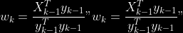 + 2. Normalize +  + to +  + 3. 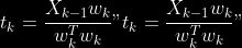 + 4. 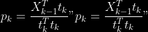 + 5.  + 6. 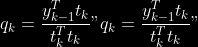 + 7.  + 8.  +**Comment** When there isn’t any missing data, stages + +and + +could be replaced by + +and + +by + +To get + so +that + +we compute : +^{-1}") +where +![\widetilde{\mathbf{P}}\_{K \times p}=\mathbf{t}\left\[p\_{1}, \ldots, p\_{K}\right\]](https://latex.codecogs.com/png.image?%5Cbg_black&space;%5Cwidetilde%7B%5Cmathbf%7BP%7D%7D_%7BK%20%5Ctimes%20p%7D%3D%5Cmathbf%7Bt%7D%5Cleft%5Bp_%7B1%7D%2C%20%5Cldots%2C%20p_%7BK%7D%5Cright%5D "\widetilde{\mathbf{P}}_{K \times p}=\mathbf{t}\left[p_{1}, \ldots, p_{K}\right]") +where +![\mathbf{W}^{\*}\_{p \times K} = \[w_1, \ldots, w_K\]](https://latex.codecogs.com/png.image?%5Cbg_black&space;%5Cmathbf%7BW%7D%5E%7B%2A%7D_%7Bp%20%5Ctimes%20K%7D%20%3D%20%5Bw_1%2C%20%5Cldots%2C%20w_K%5D "\mathbf{W}^{*}_{p \times K} = [w_1, \ldots, w_K]") +# TODO +## Input/Output +- [x] Integrate hdf5 (or exdir? msgpack?) routines to save/load + reftables/observed stats with associated metadata +- [ ] Provide R code to save/load the data +- [x] Provide Python code to save/load the data +## C++ standalone +- [x] Merge the two methodologies in a single executable with the + (almost) the same options +- [ ] (Optional) Possibly move to another options parser (CLI?) +## External interfaces +- [ ] R package +- [x] Python package +## Documentation +- [ ] Code documentation +- [ ] Document the build +## Continuous integration +- [x] Linux CI build with intel/MKL optimizations +- [x] osX CI build +- [x] Windows CI build +## Long/Mid term TODO +- methodologies parameters auto-tuning + - auto-discovering the optimal number of trees by monitoring OOB error + - auto-limiting number of threads by available memory +- Streamline the two methodologies (model choice and then parameters + estimation) +- Write our own tree/rf implementation with better storage efficiency + than ranger +- Make functional tests for the two methodologies +- Possible to use mondrian forests for online batches ? See + ([Lakshminarayanan, Roy, and Teh + 2014](#ref-lakshminarayanan2014mondrian)) +# References +This have been the subject of a proceedings in [JOBIM +2020](https://jobim2020.sciencesconf.org/), +[PDF](https://hal.archives-ouvertes.fr/hal-02910067v2) and +[video](https://relaiswebcasting.mediasite.com/mediasite/Play/8ddb4e40fc88422481f1494cf6af2bb71d?catalog=e534823f0c954836bf85bfa80af2290921) +(in french), ([Collin et al. 2020](#ref-collin:hal-02910067)). +<div id="refs" class="references csl-bib-body hanging-indent"> +<div id="ref-Collin_2021" class="csl-entry"> +Collin, François-David, Ghislain Durif, Louis Raynal, Eric Lombaert, +Mathieu Gautier, Renaud Vitalis, Jean-Michel Marin, and Arnaud Estoup. +2021. “Extending Approximate Bayesian Computation with Supervised +Machine Learning to Infer Demographic History from Genetic Polymorphisms +Using DIYABC Random Forest.” *Molecular Ecology Resources* 21 (8): +2598–2613. https://doi.org/<https://doi.org/10.1111/1755-0998.13413>. +</div> +<div id="ref-collin:hal-02910067" class="csl-entry"> +Collin, François-David, Arnaud Estoup, Jean-Michel Marin, and Louis +Raynal. 2020. “<span class="nocase">Bringing ABC inference to the +machine learning realm : AbcRanger, an optimized random forests library +for ABC</span>.” In *JOBIM 2020*, 2020:66. JOBIM. Montpellier, France. +<https://hal.archives-ouvertes.fr/hal-02910067>. +</div> +<div id="ref-friedman2001elements" class="csl-entry"> +Friedman, Jerome, Trevor Hastie, and Robert Tibshirani. 2001. *The +Elements of Statistical Learning*. Vol. 1. 10. Springer series in +statistics New York, NY, USA: +</div> +<div id="ref-eigenweb" class="csl-entry"> +Guennebaud, Gaël, Benoît Jacob, et al. 2010. “Eigen V3.” +http://eigen.tuxfamily.org. +</div> +<div id="ref-lakshminarayanan2014mondrian" class="csl-entry"> +Lakshminarayanan, Balaji, Daniel M Roy, and Yee Whye Teh. 2014. +“Mondrian Forests: Efficient Online Random Forests.” In *Advances in +Neural Information Processing Systems*, 3140–48. +</div> +<div id="ref-JMLR:v19:17-374" class="csl-entry"> +Lintusaari, Jarno, Henri Vuollekoski, Antti Kangasrääsiö, Kusti Skytén, +Marko Järvenpää, Pekka Marttinen, Michael U. Gutmann, Aki Vehtari, Jukka +Corander, and Samuel Kaski. 2018. “ELFI: Engine for Likelihood-Free +Inference.” *Journal of Machine Learning Research* 19 (16): 1–7. +<http://jmlr.org/papers/v19/17-374.html>. +</div> +<div id="ref-pudlo2015reliable" class="csl-entry"> +Pudlo, Pierre, Jean-Michel Marin, Arnaud Estoup, Jean-Marie Cornuet, +Mathieu Gautier, and Christian P Robert. 2015. “Reliable ABC Model +Choice via Random Forests.” *Bioinformatics* 32 (6): 859–66. +</div> +<div id="ref-raynal2016abc" class="csl-entry"> +Raynal, Louis, Jean-Michel Marin, Pierre Pudlo, Mathieu Ribatet, +Christian P Robert, and Arnaud Estoup. 2018. “<span class="nocase">ABC +random forests for Bayesian parameter inference</span>.” +*Bioinformatics* 35 (10): 1720–28. +<https://doi.org/10.1093/bioinformatics/bty867>. +</div> +<div id="ref-wright2015ranger" class="csl-entry"> +Wright, Marvin N, and Andreas Ziegler. 2015. “Ranger: A Fast +Implementation of Random Forests for High Dimensional Data in c++ and +r.” *arXiv Preprint arXiv:1508.04409*. +</div> +</div> +[^1]: The term “online” there and in the code has not the usual meaning + it has, as coined in “online machine learning”. We still need the + entire training data set at once. Our implementation is an “online” + one not by the sequential order of the input data, but by the + sequential order of computation of the trees in random forests, + sequentially computed and then discarded. +[^2]: We only use the C++ Core of ranger, which is under [MIT + License](https://raw.githubusercontent.com/imbs-hl/ranger/master/cpp_version/COPYING), + same as ours. + +%package -n python3-pyabcranger +Summary: ABC random forests for model choice and parameter estimation, python wrapper +Provides: python-pyabcranger +BuildRequires: python3-devel +BuildRequires: python3-setuptools +BuildRequires: python3-pip +BuildRequires: python3-cffi +BuildRequires: gcc +BuildRequires: gdb +%description -n python3-pyabcranger +- <a href="#python" id="toc-python">Python</a> +- <a href="#usage" id="toc-usage">Usage</a> +- <a href="#model-choice" id="toc-model-choice">Model Choice</a> +- <a href="#parameter-estimation" id="toc-parameter-estimation">Parameter + Estimation</a> +- <a href="#various" id="toc-various">Various</a> +- <a href="#todo" id="toc-todo">TODO</a> +- <a href="#references" id="toc-references">References</a> +<!-- pandoc -f markdown README-ORIG.md -t gfm -o README.md --citeproc -s --toc --toc-depth=1 --webtex --> +[](https://pypi.python.org/pypi/pyabcranger) +[](https://github.com/diyabc/abcranger/actions?query=workflow%3Aabcranger-build+branch%3Amaster) +Random forests methodologies for : +- ABC model choice ([Pudlo et al. 2015](#ref-pudlo2015reliable)) +- ABC Bayesian parameter inference ([Raynal et al. + 2018](#ref-raynal2016abc)) +Libraries we use : +- [Ranger](https://github.com/imbs-hl/ranger) ([Wright and Ziegler + 2015](#ref-wright2015ranger)) : we use our own fork and have tuned + forests to do “online”[^1] computations (Growing trees AND making + predictions in the same pass, which removes the need of in-memory + storage of the whole forest)[^2]. +- [Eigen3](http://eigen.tuxfamily.org) ([Guennebaud, Jacob, et al. + 2010](#ref-eigenweb)) +As a mention, we use our own implementation of LDA and PLS from +([Friedman, Hastie, and Tibshirani 2001, 1:81, +114](#ref-friedman2001elements)), PLS is optimized for univariate, see +[5.1](#sec-plsalgo). For linear algebra optimization purposes on large +reftables, the Linux version of binaries (standalone and python wheel) +are statically linked with [Intel’s Math Kernel +Library](https://www.intel.com/content/www/us/en/develop/documentation/oneapi-programming-guide/top/api-based-programming/intel-oneapi-math-kernel-library-onemkl.html), +in order to leverage multicore and SIMD extensions on modern cpus. +There is one set of binaries, which contains a Macos/Linux/Windows (x64 +only) binary for each platform. There are available within the +“[Releases](https://github.com/fradav/abcranger/releases)” tab, under +“Assets” section (unfold it to see the list). +This is pure command line binary, and they are no prerequisites or +library dependencies in order to run it. Just download them and launch +them from your terminal software of choice. The usual caveats with +command line executable apply there : if you’re not proficient with the +command line interface of your platform, please learn some basics or ask +someone who might help you in those matters. +The standalone is part of a specialized Population Genetics graphical +interface [DIYABC-RF](https://diyabc.github.io/), presented in MER +(Molecular Ecology Resources, Special Issue), ([Collin et al. +2021](#ref-Collin_2021)). +# Python +## Installation +``` bash +pip install pyabcranger +``` +## Notebooks examples +- On a [toy example with + ")](https://github.com/diyabc/abcranger/blob/master/notebooks/Toy%20example%20MA(q).ipynb), + using ([Lintusaari et al. 2018](#ref-JMLR:v19:17-374)) as + graph-powered engine. +- [Population genetics + demo](https://github.com/diyabc/abcranger/blob/master/notebooks/Population%20genetics%20Demo.ipynb), + data from ([Collin et al. 2021](#ref-Collin_2021)), available + [there](https://github.com/diyabc/diyabc/tree/master/diyabc-tests/MER/modelchoice/IndSeq) +# Usage +``` text + - ABC Random Forest - Model choice or parameter estimation command line options +Usage: + -h, --header arg Header file (default: headerRF.txt) + -r, --reftable arg Reftable file (default: reftableRF.bin) + -b, --statobs arg Statobs file (default: statobsRF.txt) + -o, --output arg Prefix output (modelchoice_out or estimparam_out by + default) + -n, --nref arg Number of samples, 0 means all (default: 0) + -m, --minnodesize arg Minimal node size. 0 means 1 for classification or + 5 for regression (default: 0) + -t, --ntree arg Number of trees (default: 500) + -j, --threads arg Number of threads, 0 means all (default: 0) + -s, --seed arg Seed, generated by default (default: 0) + -c, --noisecolumns arg Number of noise columns (default: 5) + --nolinear Disable LDA for model choice or PLS for parameter + estimation + --plsmaxvar arg Percentage of maximum explained Y-variance for + retaining pls axis (default: 0.9) + --chosenscen arg Chosen scenario (mandatory for parameter + estimation) + --noob arg number of oob testing samples (mandatory for + parameter estimation) + --parameter arg name of the parameter of interest (mandatory for + parameter estimation) + -g, --groups arg Groups of models + --help Print help +``` +- If you provide `--chosenscen`, `--parameter` and `--noob`, parameter + estimation mode is selected. +- Otherwise by default it’s model choice mode. +- Linear additions are LDA for model choice and PLS for parameter + estimation, “–nolinear” options disables them in both case. +# Model Choice + +## Example +Example : +`abcranger -t 10000 -j 8` +Header, reftable and statobs files should be in the current directory. +## Groups +With the option `-g` (or `--groups`), you may “group” your models in +several groups splitted . For example if you have six models, labeled +from 1 to 6 \`-g “1,2,3;4,5,6” +## Generated files +Four files are created : +- `modelchoice_out.ooberror` : OOB Error rate vs number of trees (line + number is the number of trees) +- `modelchoice_out.importance` : variables importance (sorted) +- `modelchoice_out.predictions` : votes, prediction and posterior error + rate +- `modelchoice_out.confusion` : OOB Confusion matrix of the classifier +# Parameter Estimation + +## Composite parameters +When specifying the parameter (option `--parameter`), one may specify +simple composite parameters as division, addition or multiplication of +two existing parameters. like `t/N` or `T1+T2`. +## A note about PLS heuristic +The `--plsmaxvar` option (defaulting at 0.90) fixes the number of +selected pls axes so that we get at least the specified percentage of +maximum explained variance of the output. The explained variance of the +output of the + first +axes is defined by the R-squared of the output: +^2}}{\sum_{i=1}^{N}{(y_{i}-\hat{y})^2}}") +where + +is the output + +scored by the pls for the +th +component. So, only the + +first axis are kept, and : + +Note that if you specify 0 as `--plsmaxvar`, an “elbow” heuristic is +activiated where the following condition is tested for every computed +axis : +\left(Yvar^{k+1}-Yvar^ {k}\right)") +If this condition is true for a windows of previous axes, sized to 10% +of the total possible axis, then we stop the PLS axis computation. +In practice, we find this + +close enough to the previous + +for 99%, but it isn’t guaranteed. +## The signification of the `noob` parameter +The median global/local statistics and confidence intervals (global) +measures for parameter estimation need a number of OOB samples +(`--noob`) to be reliable (typlially 30% of the size of the dataset is +sufficient). Be aware than computing the whole set (i.e. assigning +`--noob` the same than for `--nref`) for weights predictions ([Raynal et +al. 2018](#ref-raynal2016abc)) could be very costly, memory and +cpu-wise, if your dataset is large in number of samples, so it could be +adviseable to compute them for only choose a subset of size `noob`. +## Example (parameter estimation) +Example (working with the dataset in `test/data`) : +`abcranger -t 1000 -j 8 --parameter ra --chosenscen 1 --noob 50` +Header, reftable and statobs files should be in the current directory. +## Generated files (parameter estimation) +Five files (or seven if pls activated) are created : +- `estimparam_out.ooberror` : OOB MSE rate vs number of trees (line + number is the number of trees) +- `estimparam_out.importance` : variables importance (sorted) +- `estimparam_out.predictions` : expectation, variance and 0.05, 0.5, + 0.95 quantile for prediction +- `estimparam_out.predweights` : csv of the value/weights pairs of the + prediction (for density plot) +- `estimparam_out.oobstats` : various statistics on oob (MSE, NMSE, NMAE + etc.) +if pls enabled : +- `estimparam_out.plsvar` : variance explained by number of components +- `estimparam_out.plsweights` : variable weight in the first component + (sorted by absolute value) +# Various +## Partial Least Squares algorithm +1.  +2. For +  + 1.  + 2. Normalize +  + to +  + 3.  + 4.  + 5.  + 6.  + 7.  + 8.  +**Comment** When there isn’t any missing data, stages + +and + +could be replaced by + +and + +by + +To get + so +that + +we compute : +^{-1}") +where +![\widetilde{\mathbf{P}}\_{K \times p}=\mathbf{t}\left\[p\_{1}, \ldots, p\_{K}\right\]](https://latex.codecogs.com/png.image?%5Cbg_black&space;%5Cwidetilde%7B%5Cmathbf%7BP%7D%7D_%7BK%20%5Ctimes%20p%7D%3D%5Cmathbf%7Bt%7D%5Cleft%5Bp_%7B1%7D%2C%20%5Cldots%2C%20p_%7BK%7D%5Cright%5D "\widetilde{\mathbf{P}}_{K \times p}=\mathbf{t}\left[p_{1}, \ldots, p_{K}\right]") +where +![\mathbf{W}^{\*}\_{p \times K} = \[w_1, \ldots, w_K\]](https://latex.codecogs.com/png.image?%5Cbg_black&space;%5Cmathbf%7BW%7D%5E%7B%2A%7D_%7Bp%20%5Ctimes%20K%7D%20%3D%20%5Bw_1%2C%20%5Cldots%2C%20w_K%5D "\mathbf{W}^{*}_{p \times K} = [w_1, \ldots, w_K]") +# TODO +## Input/Output +- [x] Integrate hdf5 (or exdir? msgpack?) routines to save/load + reftables/observed stats with associated metadata +- [ ] Provide R code to save/load the data +- [x] Provide Python code to save/load the data +## C++ standalone +- [x] Merge the two methodologies in a single executable with the + (almost) the same options +- [ ] (Optional) Possibly move to another options parser (CLI?) +## External interfaces +- [ ] R package +- [x] Python package +## Documentation +- [ ] Code documentation +- [ ] Document the build +## Continuous integration +- [x] Linux CI build with intel/MKL optimizations +- [x] osX CI build +- [x] Windows CI build +## Long/Mid term TODO +- methodologies parameters auto-tuning + - auto-discovering the optimal number of trees by monitoring OOB error + - auto-limiting number of threads by available memory +- Streamline the two methodologies (model choice and then parameters + estimation) +- Write our own tree/rf implementation with better storage efficiency + than ranger +- Make functional tests for the two methodologies +- Possible to use mondrian forests for online batches ? See + ([Lakshminarayanan, Roy, and Teh + 2014](#ref-lakshminarayanan2014mondrian)) +# References +This have been the subject of a proceedings in [JOBIM +2020](https://jobim2020.sciencesconf.org/), +[PDF](https://hal.archives-ouvertes.fr/hal-02910067v2) and +[video](https://relaiswebcasting.mediasite.com/mediasite/Play/8ddb4e40fc88422481f1494cf6af2bb71d?catalog=e534823f0c954836bf85bfa80af2290921) +(in french), ([Collin et al. 2020](#ref-collin:hal-02910067)). +<div id="refs" class="references csl-bib-body hanging-indent"> +<div id="ref-Collin_2021" class="csl-entry"> +Collin, François-David, Ghislain Durif, Louis Raynal, Eric Lombaert, +Mathieu Gautier, Renaud Vitalis, Jean-Michel Marin, and Arnaud Estoup. +2021. “Extending Approximate Bayesian Computation with Supervised +Machine Learning to Infer Demographic History from Genetic Polymorphisms +Using DIYABC Random Forest.” *Molecular Ecology Resources* 21 (8): +2598–2613. https://doi.org/<https://doi.org/10.1111/1755-0998.13413>. +</div> +<div id="ref-collin:hal-02910067" class="csl-entry"> +Collin, François-David, Arnaud Estoup, Jean-Michel Marin, and Louis +Raynal. 2020. “<span class="nocase">Bringing ABC inference to the +machine learning realm : AbcRanger, an optimized random forests library +for ABC</span>.” In *JOBIM 2020*, 2020:66. JOBIM. Montpellier, France. +<https://hal.archives-ouvertes.fr/hal-02910067>. +</div> +<div id="ref-friedman2001elements" class="csl-entry"> +Friedman, Jerome, Trevor Hastie, and Robert Tibshirani. 2001. *The +Elements of Statistical Learning*. Vol. 1. 10. Springer series in +statistics New York, NY, USA: +</div> +<div id="ref-eigenweb" class="csl-entry"> +Guennebaud, Gaël, Benoît Jacob, et al. 2010. “Eigen V3.” +http://eigen.tuxfamily.org. +</div> +<div id="ref-lakshminarayanan2014mondrian" class="csl-entry"> +Lakshminarayanan, Balaji, Daniel M Roy, and Yee Whye Teh. 2014. +“Mondrian Forests: Efficient Online Random Forests.” In *Advances in +Neural Information Processing Systems*, 3140–48. +</div> +<div id="ref-JMLR:v19:17-374" class="csl-entry"> +Lintusaari, Jarno, Henri Vuollekoski, Antti Kangasrääsiö, Kusti Skytén, +Marko Järvenpää, Pekka Marttinen, Michael U. Gutmann, Aki Vehtari, Jukka +Corander, and Samuel Kaski. 2018. “ELFI: Engine for Likelihood-Free +Inference.” *Journal of Machine Learning Research* 19 (16): 1–7. +<http://jmlr.org/papers/v19/17-374.html>. +</div> +<div id="ref-pudlo2015reliable" class="csl-entry"> +Pudlo, Pierre, Jean-Michel Marin, Arnaud Estoup, Jean-Marie Cornuet, +Mathieu Gautier, and Christian P Robert. 2015. “Reliable ABC Model +Choice via Random Forests.” *Bioinformatics* 32 (6): 859–66. +</div> +<div id="ref-raynal2016abc" class="csl-entry"> +Raynal, Louis, Jean-Michel Marin, Pierre Pudlo, Mathieu Ribatet, +Christian P Robert, and Arnaud Estoup. 2018. “<span class="nocase">ABC +random forests for Bayesian parameter inference</span>.” +*Bioinformatics* 35 (10): 1720–28. +<https://doi.org/10.1093/bioinformatics/bty867>. +</div> +<div id="ref-wright2015ranger" class="csl-entry"> +Wright, Marvin N, and Andreas Ziegler. 2015. “Ranger: A Fast +Implementation of Random Forests for High Dimensional Data in c++ and +r.” *arXiv Preprint arXiv:1508.04409*. +</div> +</div> +[^1]: The term “online” there and in the code has not the usual meaning + it has, as coined in “online machine learning”. We still need the + entire training data set at once. Our implementation is an “online” + one not by the sequential order of the input data, but by the + sequential order of computation of the trees in random forests, + sequentially computed and then discarded. +[^2]: We only use the C++ Core of ranger, which is under [MIT + License](https://raw.githubusercontent.com/imbs-hl/ranger/master/cpp_version/COPYING), + same as ours. + +%package help +Summary: Development documents and examples for pyabcranger +Provides: python3-pyabcranger-doc +%description help +- <a href="#python" id="toc-python">Python</a> +- <a href="#usage" id="toc-usage">Usage</a> +- <a href="#model-choice" id="toc-model-choice">Model Choice</a> +- <a href="#parameter-estimation" id="toc-parameter-estimation">Parameter + Estimation</a> +- <a href="#various" id="toc-various">Various</a> +- <a href="#todo" id="toc-todo">TODO</a> +- <a href="#references" id="toc-references">References</a> +<!-- pandoc -f markdown README-ORIG.md -t gfm -o README.md --citeproc -s --toc --toc-depth=1 --webtex --> +[](https://pypi.python.org/pypi/pyabcranger) +[](https://github.com/diyabc/abcranger/actions?query=workflow%3Aabcranger-build+branch%3Amaster) +Random forests methodologies for : +- ABC model choice ([Pudlo et al. 2015](#ref-pudlo2015reliable)) +- ABC Bayesian parameter inference ([Raynal et al. + 2018](#ref-raynal2016abc)) +Libraries we use : +- [Ranger](https://github.com/imbs-hl/ranger) ([Wright and Ziegler + 2015](#ref-wright2015ranger)) : we use our own fork and have tuned + forests to do “online”[^1] computations (Growing trees AND making + predictions in the same pass, which removes the need of in-memory + storage of the whole forest)[^2]. +- [Eigen3](http://eigen.tuxfamily.org) ([Guennebaud, Jacob, et al. + 2010](#ref-eigenweb)) +As a mention, we use our own implementation of LDA and PLS from +([Friedman, Hastie, and Tibshirani 2001, 1:81, +114](#ref-friedman2001elements)), PLS is optimized for univariate, see +[5.1](#sec-plsalgo). For linear algebra optimization purposes on large +reftables, the Linux version of binaries (standalone and python wheel) +are statically linked with [Intel’s Math Kernel +Library](https://www.intel.com/content/www/us/en/develop/documentation/oneapi-programming-guide/top/api-based-programming/intel-oneapi-math-kernel-library-onemkl.html), +in order to leverage multicore and SIMD extensions on modern cpus. +There is one set of binaries, which contains a Macos/Linux/Windows (x64 +only) binary for each platform. There are available within the +“[Releases](https://github.com/fradav/abcranger/releases)” tab, under +“Assets” section (unfold it to see the list). +This is pure command line binary, and they are no prerequisites or +library dependencies in order to run it. Just download them and launch +them from your terminal software of choice. The usual caveats with +command line executable apply there : if you’re not proficient with the +command line interface of your platform, please learn some basics or ask +someone who might help you in those matters. +The standalone is part of a specialized Population Genetics graphical +interface [DIYABC-RF](https://diyabc.github.io/), presented in MER +(Molecular Ecology Resources, Special Issue), ([Collin et al. +2021](#ref-Collin_2021)). +# Python +## Installation +``` bash +pip install pyabcranger +``` +## Notebooks examples +- On a [toy example with + ")](https://github.com/diyabc/abcranger/blob/master/notebooks/Toy%20example%20MA(q).ipynb), + using ([Lintusaari et al. 2018](#ref-JMLR:v19:17-374)) as + graph-powered engine. +- [Population genetics + demo](https://github.com/diyabc/abcranger/blob/master/notebooks/Population%20genetics%20Demo.ipynb), + data from ([Collin et al. 2021](#ref-Collin_2021)), available + [there](https://github.com/diyabc/diyabc/tree/master/diyabc-tests/MER/modelchoice/IndSeq) +# Usage +``` text + - ABC Random Forest - Model choice or parameter estimation command line options +Usage: + -h, --header arg Header file (default: headerRF.txt) + -r, --reftable arg Reftable file (default: reftableRF.bin) + -b, --statobs arg Statobs file (default: statobsRF.txt) + -o, --output arg Prefix output (modelchoice_out or estimparam_out by + default) + -n, --nref arg Number of samples, 0 means all (default: 0) + -m, --minnodesize arg Minimal node size. 0 means 1 for classification or + 5 for regression (default: 0) + -t, --ntree arg Number of trees (default: 500) + -j, --threads arg Number of threads, 0 means all (default: 0) + -s, --seed arg Seed, generated by default (default: 0) + -c, --noisecolumns arg Number of noise columns (default: 5) + --nolinear Disable LDA for model choice or PLS for parameter + estimation + --plsmaxvar arg Percentage of maximum explained Y-variance for + retaining pls axis (default: 0.9) + --chosenscen arg Chosen scenario (mandatory for parameter + estimation) + --noob arg number of oob testing samples (mandatory for + parameter estimation) + --parameter arg name of the parameter of interest (mandatory for + parameter estimation) + -g, --groups arg Groups of models + --help Print help +``` +- If you provide `--chosenscen`, `--parameter` and `--noob`, parameter + estimation mode is selected. +- Otherwise by default it’s model choice mode. +- Linear additions are LDA for model choice and PLS for parameter + estimation, “–nolinear” options disables them in both case. +# Model Choice + +## Example +Example : +`abcranger -t 10000 -j 8` +Header, reftable and statobs files should be in the current directory. +## Groups +With the option `-g` (or `--groups`), you may “group” your models in +several groups splitted . For example if you have six models, labeled +from 1 to 6 \`-g “1,2,3;4,5,6” +## Generated files +Four files are created : +- `modelchoice_out.ooberror` : OOB Error rate vs number of trees (line + number is the number of trees) +- `modelchoice_out.importance` : variables importance (sorted) +- `modelchoice_out.predictions` : votes, prediction and posterior error + rate +- `modelchoice_out.confusion` : OOB Confusion matrix of the classifier +# Parameter Estimation + +## Composite parameters +When specifying the parameter (option `--parameter`), one may specify +simple composite parameters as division, addition or multiplication of +two existing parameters. like `t/N` or `T1+T2`. +## A note about PLS heuristic +The `--plsmaxvar` option (defaulting at 0.90) fixes the number of +selected pls axes so that we get at least the specified percentage of +maximum explained variance of the output. The explained variance of the +output of the + first +axes is defined by the R-squared of the output: +^2}}{\sum_{i=1}^{N}{(y_{i}-\hat{y})^2}}") +where + +is the output + +scored by the pls for the +th +component. So, only the + +first axis are kept, and : + +Note that if you specify 0 as `--plsmaxvar`, an “elbow” heuristic is +activiated where the following condition is tested for every computed +axis : +\left(Yvar^{k+1}-Yvar^ {k}\right)") +If this condition is true for a windows of previous axes, sized to 10% +of the total possible axis, then we stop the PLS axis computation. +In practice, we find this + +close enough to the previous + +for 99%, but it isn’t guaranteed. +## The signification of the `noob` parameter +The median global/local statistics and confidence intervals (global) +measures for parameter estimation need a number of OOB samples +(`--noob`) to be reliable (typlially 30% of the size of the dataset is +sufficient). Be aware than computing the whole set (i.e. assigning +`--noob` the same than for `--nref`) for weights predictions ([Raynal et +al. 2018](#ref-raynal2016abc)) could be very costly, memory and +cpu-wise, if your dataset is large in number of samples, so it could be +adviseable to compute them for only choose a subset of size `noob`. +## Example (parameter estimation) +Example (working with the dataset in `test/data`) : +`abcranger -t 1000 -j 8 --parameter ra --chosenscen 1 --noob 50` +Header, reftable and statobs files should be in the current directory. +## Generated files (parameter estimation) +Five files (or seven if pls activated) are created : +- `estimparam_out.ooberror` : OOB MSE rate vs number of trees (line + number is the number of trees) +- `estimparam_out.importance` : variables importance (sorted) +- `estimparam_out.predictions` : expectation, variance and 0.05, 0.5, + 0.95 quantile for prediction +- `estimparam_out.predweights` : csv of the value/weights pairs of the + prediction (for density plot) +- `estimparam_out.oobstats` : various statistics on oob (MSE, NMSE, NMAE + etc.) +if pls enabled : +- `estimparam_out.plsvar` : variance explained by number of components +- `estimparam_out.plsweights` : variable weight in the first component + (sorted by absolute value) +# Various +## Partial Least Squares algorithm +1.  +2. For +  + 1.  + 2. Normalize +  + to +  + 3.  + 4.  + 5.  + 6.  + 7.  + 8.  +**Comment** When there isn’t any missing data, stages + +and + +could be replaced by + +and + +by + +To get + so +that + +we compute : +^{-1}") +where +![\widetilde{\mathbf{P}}\_{K \times p}=\mathbf{t}\left\[p\_{1}, \ldots, p\_{K}\right\]](https://latex.codecogs.com/png.image?%5Cbg_black&space;%5Cwidetilde%7B%5Cmathbf%7BP%7D%7D_%7BK%20%5Ctimes%20p%7D%3D%5Cmathbf%7Bt%7D%5Cleft%5Bp_%7B1%7D%2C%20%5Cldots%2C%20p_%7BK%7D%5Cright%5D "\widetilde{\mathbf{P}}_{K \times p}=\mathbf{t}\left[p_{1}, \ldots, p_{K}\right]") +where +![\mathbf{W}^{\*}\_{p \times K} = \[w_1, \ldots, w_K\]](https://latex.codecogs.com/png.image?%5Cbg_black&space;%5Cmathbf%7BW%7D%5E%7B%2A%7D_%7Bp%20%5Ctimes%20K%7D%20%3D%20%5Bw_1%2C%20%5Cldots%2C%20w_K%5D "\mathbf{W}^{*}_{p \times K} = [w_1, \ldots, w_K]") +# TODO +## Input/Output +- [x] Integrate hdf5 (or exdir? msgpack?) routines to save/load + reftables/observed stats with associated metadata +- [ ] Provide R code to save/load the data +- [x] Provide Python code to save/load the data +## C++ standalone +- [x] Merge the two methodologies in a single executable with the + (almost) the same options +- [ ] (Optional) Possibly move to another options parser (CLI?) +## External interfaces +- [ ] R package +- [x] Python package +## Documentation +- [ ] Code documentation +- [ ] Document the build +## Continuous integration +- [x] Linux CI build with intel/MKL optimizations +- [x] osX CI build +- [x] Windows CI build +## Long/Mid term TODO +- methodologies parameters auto-tuning + - auto-discovering the optimal number of trees by monitoring OOB error + - auto-limiting number of threads by available memory +- Streamline the two methodologies (model choice and then parameters + estimation) +- Write our own tree/rf implementation with better storage efficiency + than ranger +- Make functional tests for the two methodologies +- Possible to use mondrian forests for online batches ? See + ([Lakshminarayanan, Roy, and Teh + 2014](#ref-lakshminarayanan2014mondrian)) +# References +This have been the subject of a proceedings in [JOBIM +2020](https://jobim2020.sciencesconf.org/), +[PDF](https://hal.archives-ouvertes.fr/hal-02910067v2) and +[video](https://relaiswebcasting.mediasite.com/mediasite/Play/8ddb4e40fc88422481f1494cf6af2bb71d?catalog=e534823f0c954836bf85bfa80af2290921) +(in french), ([Collin et al. 2020](#ref-collin:hal-02910067)). +<div id="refs" class="references csl-bib-body hanging-indent"> +<div id="ref-Collin_2021" class="csl-entry"> +Collin, François-David, Ghislain Durif, Louis Raynal, Eric Lombaert, +Mathieu Gautier, Renaud Vitalis, Jean-Michel Marin, and Arnaud Estoup. +2021. “Extending Approximate Bayesian Computation with Supervised +Machine Learning to Infer Demographic History from Genetic Polymorphisms +Using DIYABC Random Forest.” *Molecular Ecology Resources* 21 (8): +2598–2613. https://doi.org/<https://doi.org/10.1111/1755-0998.13413>. +</div> +<div id="ref-collin:hal-02910067" class="csl-entry"> +Collin, François-David, Arnaud Estoup, Jean-Michel Marin, and Louis +Raynal. 2020. “<span class="nocase">Bringing ABC inference to the +machine learning realm : AbcRanger, an optimized random forests library +for ABC</span>.” In *JOBIM 2020*, 2020:66. JOBIM. Montpellier, France. +<https://hal.archives-ouvertes.fr/hal-02910067>. +</div> +<div id="ref-friedman2001elements" class="csl-entry"> +Friedman, Jerome, Trevor Hastie, and Robert Tibshirani. 2001. *The +Elements of Statistical Learning*. Vol. 1. 10. Springer series in +statistics New York, NY, USA: +</div> +<div id="ref-eigenweb" class="csl-entry"> +Guennebaud, Gaël, Benoît Jacob, et al. 2010. “Eigen V3.” +http://eigen.tuxfamily.org. +</div> +<div id="ref-lakshminarayanan2014mondrian" class="csl-entry"> +Lakshminarayanan, Balaji, Daniel M Roy, and Yee Whye Teh. 2014. +“Mondrian Forests: Efficient Online Random Forests.” In *Advances in +Neural Information Processing Systems*, 3140–48. +</div> +<div id="ref-JMLR:v19:17-374" class="csl-entry"> +Lintusaari, Jarno, Henri Vuollekoski, Antti Kangasrääsiö, Kusti Skytén, +Marko Järvenpää, Pekka Marttinen, Michael U. Gutmann, Aki Vehtari, Jukka +Corander, and Samuel Kaski. 2018. “ELFI: Engine for Likelihood-Free +Inference.” *Journal of Machine Learning Research* 19 (16): 1–7. +<http://jmlr.org/papers/v19/17-374.html>. +</div> +<div id="ref-pudlo2015reliable" class="csl-entry"> +Pudlo, Pierre, Jean-Michel Marin, Arnaud Estoup, Jean-Marie Cornuet, +Mathieu Gautier, and Christian P Robert. 2015. “Reliable ABC Model +Choice via Random Forests.” *Bioinformatics* 32 (6): 859–66. +</div> +<div id="ref-raynal2016abc" class="csl-entry"> +Raynal, Louis, Jean-Michel Marin, Pierre Pudlo, Mathieu Ribatet, +Christian P Robert, and Arnaud Estoup. 2018. “<span class="nocase">ABC +random forests for Bayesian parameter inference</span>.” +*Bioinformatics* 35 (10): 1720–28. +<https://doi.org/10.1093/bioinformatics/bty867>. +</div> +<div id="ref-wright2015ranger" class="csl-entry"> +Wright, Marvin N, and Andreas Ziegler. 2015. “Ranger: A Fast +Implementation of Random Forests for High Dimensional Data in c++ and +r.” *arXiv Preprint arXiv:1508.04409*. +</div> +</div> +[^1]: The term “online” there and in the code has not the usual meaning + it has, as coined in “online machine learning”. We still need the + entire training data set at once. Our implementation is an “online” + one not by the sequential order of the input data, but by the + sequential order of computation of the trees in random forests, + sequentially computed and then discarded. +[^2]: We only use the C++ Core of ranger, which is under [MIT + License](https://raw.githubusercontent.com/imbs-hl/ranger/master/cpp_version/COPYING), + same as ours. + +%prep +%autosetup -n pyabcranger-0.0.69 + +%build +%py3_build + +%install +%py3_install +install -d -m755 %{buildroot}/%{_pkgdocdir} +if [ -d doc ]; then cp -arf doc %{buildroot}/%{_pkgdocdir}; fi +if [ -d docs ]; then cp -arf docs %{buildroot}/%{_pkgdocdir}; fi +if [ -d example ]; then cp -arf example %{buildroot}/%{_pkgdocdir}; fi +if [ -d examples ]; then cp -arf examples %{buildroot}/%{_pkgdocdir}; fi +pushd %{buildroot} +if [ -d usr/lib ]; then + find usr/lib -type f -printf "/%h/%f\n" >> filelist.lst +fi +if [ -d usr/lib64 ]; then + find usr/lib64 -type f -printf "/%h/%f\n" >> filelist.lst +fi +if [ -d usr/bin ]; then + find usr/bin -type f -printf "/%h/%f\n" >> filelist.lst +fi +if [ -d usr/sbin ]; then + find usr/sbin -type f -printf "/%h/%f\n" >> filelist.lst +fi +touch doclist.lst +if [ -d usr/share/man ]; then + find usr/share/man -type f -printf "/%h/%f.gz\n" >> doclist.lst +fi +popd +mv %{buildroot}/filelist.lst . +mv %{buildroot}/doclist.lst . + +%files -n python3-pyabcranger -f filelist.lst +%dir %{python3_sitearch}/* + +%files help -f doclist.lst +%{_docdir}/* + +%changelog +* Mon May 29 2023 Python_Bot <Python_Bot@openeuler.org> - 0.0.69-1 +- Package Spec generated @@ -0,0 +1 @@ +d753357721d022bbe691c3f19aa6a7c0 pyabcranger-0.0.69.tar.gz |