%global _empty_manifest_terminate_build 0
Name: python-pyabcranger
Version: 0.0.69
Release: 1
Summary: ABC random forests for model choice and parameter estimation, python wrapper
License: MIT License
URL: https://github.com/diyabc/abcranger
Source0: https://mirrors.nju.edu.cn/pypi/web/packages/47/37/21ddd826ccf085c31879705a0b283dd3f16e0712ce8563d325e786b7ed7b/pyabcranger-0.0.69.tar.gz
%description
- Python
- Usage
- Model Choice
- Parameter
Estimation
- Various
- TODO
- References
[](https://pypi.python.org/pypi/pyabcranger)
[](https://github.com/diyabc/abcranger/actions?query=workflow%3Aabcranger-build+branch%3Amaster)
Random forests methodologies for :
- ABC model choice ([Pudlo et al. 2015](#ref-pudlo2015reliable))
- ABC Bayesian parameter inference ([Raynal et al.
2018](#ref-raynal2016abc))
Libraries we use :
- [Ranger](https://github.com/imbs-hl/ranger) ([Wright and Ziegler
2015](#ref-wright2015ranger)) : we use our own fork and have tuned
forests to do “online”[^1] computations (Growing trees AND making
predictions in the same pass, which removes the need of in-memory
storage of the whole forest)[^2].
- [Eigen3](http://eigen.tuxfamily.org) ([Guennebaud, Jacob, et al.
2010](#ref-eigenweb))
As a mention, we use our own implementation of LDA and PLS from
([Friedman, Hastie, and Tibshirani 2001, 1:81,
114](#ref-friedman2001elements)), PLS is optimized for univariate, see
[5.1](#sec-plsalgo). For linear algebra optimization purposes on large
reftables, the Linux version of binaries (standalone and python wheel)
are statically linked with [Intel’s Math Kernel
Library](https://www.intel.com/content/www/us/en/develop/documentation/oneapi-programming-guide/top/api-based-programming/intel-oneapi-math-kernel-library-onemkl.html),
in order to leverage multicore and SIMD extensions on modern cpus.
There is one set of binaries, which contains a Macos/Linux/Windows (x64
only) binary for each platform. There are available within the
“[Releases](https://github.com/fradav/abcranger/releases)” tab, under
“Assets” section (unfold it to see the list).
This is pure command line binary, and they are no prerequisites or
library dependencies in order to run it. Just download them and launch
them from your terminal software of choice. The usual caveats with
command line executable apply there : if you’re not proficient with the
command line interface of your platform, please learn some basics or ask
someone who might help you in those matters.
The standalone is part of a specialized Population Genetics graphical
interface [DIYABC-RF](https://diyabc.github.io/), presented in MER
(Molecular Ecology Resources, Special Issue), ([Collin et al.
2021](#ref-Collin_2021)).
# Python
## Installation
``` bash
pip install pyabcranger
```
## Notebooks examples
- On a [toy example with
")](https://github.com/diyabc/abcranger/blob/master/notebooks/Toy%20example%20MA(q).ipynb),
using ([Lintusaari et al. 2018](#ref-JMLR:v19:17-374)) as
graph-powered engine.
- [Population genetics
demo](https://github.com/diyabc/abcranger/blob/master/notebooks/Population%20genetics%20Demo.ipynb),
data from ([Collin et al. 2021](#ref-Collin_2021)), available
[there](https://github.com/diyabc/diyabc/tree/master/diyabc-tests/MER/modelchoice/IndSeq)
# Usage
``` text
- ABC Random Forest - Model choice or parameter estimation command line options
Usage:
-h, --header arg Header file (default: headerRF.txt)
-r, --reftable arg Reftable file (default: reftableRF.bin)
-b, --statobs arg Statobs file (default: statobsRF.txt)
-o, --output arg Prefix output (modelchoice_out or estimparam_out by
default)
-n, --nref arg Number of samples, 0 means all (default: 0)
-m, --minnodesize arg Minimal node size. 0 means 1 for classification or
5 for regression (default: 0)
-t, --ntree arg Number of trees (default: 500)
-j, --threads arg Number of threads, 0 means all (default: 0)
-s, --seed arg Seed, generated by default (default: 0)
-c, --noisecolumns arg Number of noise columns (default: 5)
--nolinear Disable LDA for model choice or PLS for parameter
estimation
--plsmaxvar arg Percentage of maximum explained Y-variance for
retaining pls axis (default: 0.9)
--chosenscen arg Chosen scenario (mandatory for parameter
estimation)
--noob arg number of oob testing samples (mandatory for
parameter estimation)
--parameter arg name of the parameter of interest (mandatory for
parameter estimation)
-g, --groups arg Groups of models
--help Print help
```
- If you provide `--chosenscen`, `--parameter` and `--noob`, parameter
estimation mode is selected.
- Otherwise by default it’s model choice mode.
- Linear additions are LDA for model choice and PLS for parameter
estimation, “–nolinear” options disables them in both case.
# Model Choice

## Example
Example :
`abcranger -t 10000 -j 8`
Header, reftable and statobs files should be in the current directory.
## Groups
With the option `-g` (or `--groups`), you may “group” your models in
several groups splitted . For example if you have six models, labeled
from 1 to 6 \`-g “1,2,3;4,5,6”
## Generated files
Four files are created :
- `modelchoice_out.ooberror` : OOB Error rate vs number of trees (line
number is the number of trees)
- `modelchoice_out.importance` : variables importance (sorted)
- `modelchoice_out.predictions` : votes, prediction and posterior error
rate
- `modelchoice_out.confusion` : OOB Confusion matrix of the classifier
# Parameter Estimation

## Composite parameters
When specifying the parameter (option `--parameter`), one may specify
simple composite parameters as division, addition or multiplication of
two existing parameters. like `t/N` or `T1+T2`.
## A note about PLS heuristic
The `--plsmaxvar` option (defaulting at 0.90) fixes the number of
selected pls axes so that we get at least the specified percentage of
maximum explained variance of the output. The explained variance of the
output of the
 first
axes is defined by the R-squared of the output:
^2}}{\sum_{i=1}^{N}{(y_{i}-\hat{y})^2}}")
where

is the output

scored by the pls for the
th
component. So, only the

first axis are kept, and :

Note that if you specify 0 as `--plsmaxvar`, an “elbow” heuristic is
activiated where the following condition is tested for every computed
axis :
\left(Yvar^{k+1}-Yvar^ {k}\right)")
If this condition is true for a windows of previous axes, sized to 10%
of the total possible axis, then we stop the PLS axis computation.
In practice, we find this

close enough to the previous

for 99%, but it isn’t guaranteed.
## The signification of the `noob` parameter
The median global/local statistics and confidence intervals (global)
measures for parameter estimation need a number of OOB samples
(`--noob`) to be reliable (typlially 30% of the size of the dataset is
sufficient). Be aware than computing the whole set (i.e. assigning
`--noob` the same than for `--nref`) for weights predictions ([Raynal et
al. 2018](#ref-raynal2016abc)) could be very costly, memory and
cpu-wise, if your dataset is large in number of samples, so it could be
adviseable to compute them for only choose a subset of size `noob`.
## Example (parameter estimation)
Example (working with the dataset in `test/data`) :
`abcranger -t 1000 -j 8 --parameter ra --chosenscen 1 --noob 50`
Header, reftable and statobs files should be in the current directory.
## Generated files (parameter estimation)
Five files (or seven if pls activated) are created :
- `estimparam_out.ooberror` : OOB MSE rate vs number of trees (line
number is the number of trees)
- `estimparam_out.importance` : variables importance (sorted)
- `estimparam_out.predictions` : expectation, variance and 0.05, 0.5,
0.95 quantile for prediction
- `estimparam_out.predweights` : csv of the value/weights pairs of the
prediction (for density plot)
- `estimparam_out.oobstats` : various statistics on oob (MSE, NMSE, NMAE
etc.)
if pls enabled :
- `estimparam_out.plsvar` : variance explained by number of components
- `estimparam_out.plsweights` : variable weight in the first component
(sorted by absolute value)
# Various
## Partial Least Squares algorithm
1. 
2. For

1. 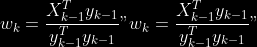
2. Normalize

to

3. 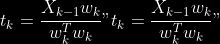
4. 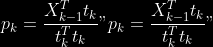
5. 
6. 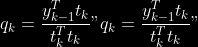
7. 
8. 
**Comment** When there isn’t any missing data, stages

and

could be replaced by
and

by

To get
 so
that

we compute :
^{-1}")
where
![\widetilde{\mathbf{P}}\_{K \times p}=\mathbf{t}\left\[p\_{1}, \ldots, p\_{K}\right\]](https://latex.codecogs.com/png.image?%5Cbg_black&space;%5Cwidetilde%7B%5Cmathbf%7BP%7D%7D_%7BK%20%5Ctimes%20p%7D%3D%5Cmathbf%7Bt%7D%5Cleft%5Bp_%7B1%7D%2C%20%5Cldots%2C%20p_%7BK%7D%5Cright%5D "\widetilde{\mathbf{P}}_{K \times p}=\mathbf{t}\left[p_{1}, \ldots, p_{K}\right]")
where
![\mathbf{W}^{\*}\_{p \times K} = \[w_1, \ldots, w_K\]](https://latex.codecogs.com/png.image?%5Cbg_black&space;%5Cmathbf%7BW%7D%5E%7B%2A%7D_%7Bp%20%5Ctimes%20K%7D%20%3D%20%5Bw_1%2C%20%5Cldots%2C%20w_K%5D "\mathbf{W}^{*}_{p \times K} = [w_1, \ldots, w_K]")
# TODO
## Input/Output
- [x] Integrate hdf5 (or exdir? msgpack?) routines to save/load
reftables/observed stats with associated metadata
- [ ] Provide R code to save/load the data
- [x] Provide Python code to save/load the data
## C++ standalone
- [x] Merge the two methodologies in a single executable with the
(almost) the same options
- [ ] (Optional) Possibly move to another options parser (CLI?)
## External interfaces
- [ ] R package
- [x] Python package
## Documentation
- [ ] Code documentation
- [ ] Document the build
## Continuous integration
- [x] Linux CI build with intel/MKL optimizations
- [x] osX CI build
- [x] Windows CI build
## Long/Mid term TODO
- methodologies parameters auto-tuning
- auto-discovering the optimal number of trees by monitoring OOB error
- auto-limiting number of threads by available memory
- Streamline the two methodologies (model choice and then parameters
estimation)
- Write our own tree/rf implementation with better storage efficiency
than ranger
- Make functional tests for the two methodologies
- Possible to use mondrian forests for online batches ? See
([Lakshminarayanan, Roy, and Teh
2014](#ref-lakshminarayanan2014mondrian))
# References
This have been the subject of a proceedings in [JOBIM
2020](https://jobim2020.sciencesconf.org/),
[PDF](https://hal.archives-ouvertes.fr/hal-02910067v2) and
[video](https://relaiswebcasting.mediasite.com/mediasite/Play/8ddb4e40fc88422481f1494cf6af2bb71d?catalog=e534823f0c954836bf85bfa80af2290921)
(in french), ([Collin et al. 2020](#ref-collin:hal-02910067)).
Collin, François-David, Ghislain Durif, Louis Raynal, Eric Lombaert,
Mathieu Gautier, Renaud Vitalis, Jean-Michel Marin, and Arnaud Estoup.
2021. “Extending Approximate Bayesian Computation with Supervised
Machine Learning to Infer Demographic History from Genetic Polymorphisms
Using DIYABC Random Forest.” *Molecular Ecology Resources* 21 (8):
2598–2613. https://doi.org/.
Collin, François-David, Arnaud Estoup, Jean-Michel Marin, and Louis
Raynal. 2020. “Bringing ABC inference to the
machine learning realm : AbcRanger, an optimized random forests library
for ABC.” In *JOBIM 2020*, 2020:66. JOBIM. Montpellier, France.
.
Friedman, Jerome, Trevor Hastie, and Robert Tibshirani. 2001. *The
Elements of Statistical Learning*. Vol. 1. 10. Springer series in
statistics New York, NY, USA:
Guennebaud, Gaël, Benoît Jacob, et al. 2010. “Eigen V3.”
http://eigen.tuxfamily.org.
Lakshminarayanan, Balaji, Daniel M Roy, and Yee Whye Teh. 2014.
“Mondrian Forests: Efficient Online Random Forests.” In *Advances in
Neural Information Processing Systems*, 3140–48.
Lintusaari, Jarno, Henri Vuollekoski, Antti Kangasrääsiö, Kusti Skytén,
Marko Järvenpää, Pekka Marttinen, Michael U. Gutmann, Aki Vehtari, Jukka
Corander, and Samuel Kaski. 2018. “ELFI: Engine for Likelihood-Free
Inference.” *Journal of Machine Learning Research* 19 (16): 1–7.
.
Pudlo, Pierre, Jean-Michel Marin, Arnaud Estoup, Jean-Marie Cornuet,
Mathieu Gautier, and Christian P Robert. 2015. “Reliable ABC Model
Choice via Random Forests.” *Bioinformatics* 32 (6): 859–66.
Raynal, Louis, Jean-Michel Marin, Pierre Pudlo, Mathieu Ribatet,
Christian P Robert, and Arnaud Estoup. 2018. “ABC
random forests for Bayesian parameter inference.”
*Bioinformatics* 35 (10): 1720–28.
.
Wright, Marvin N, and Andreas Ziegler. 2015. “Ranger: A Fast
Implementation of Random Forests for High Dimensional Data in c++ and
r.” *arXiv Preprint arXiv:1508.04409*.
[^1]: The term “online” there and in the code has not the usual meaning
it has, as coined in “online machine learning”. We still need the
entire training data set at once. Our implementation is an “online”
one not by the sequential order of the input data, but by the
sequential order of computation of the trees in random forests,
sequentially computed and then discarded.
[^2]: We only use the C++ Core of ranger, which is under [MIT
License](https://raw.githubusercontent.com/imbs-hl/ranger/master/cpp_version/COPYING),
same as ours.
%package -n python3-pyabcranger
Summary: ABC random forests for model choice and parameter estimation, python wrapper
Provides: python-pyabcranger
BuildRequires: python3-devel
BuildRequires: python3-setuptools
BuildRequires: python3-pip
BuildRequires: python3-cffi
BuildRequires: gcc
BuildRequires: gdb
%description -n python3-pyabcranger
- Python
- Usage
- Model Choice
- Parameter
Estimation
- Various
- TODO
- References
[](https://pypi.python.org/pypi/pyabcranger)
[](https://github.com/diyabc/abcranger/actions?query=workflow%3Aabcranger-build+branch%3Amaster)
Random forests methodologies for :
- ABC model choice ([Pudlo et al. 2015](#ref-pudlo2015reliable))
- ABC Bayesian parameter inference ([Raynal et al.
2018](#ref-raynal2016abc))
Libraries we use :
- [Ranger](https://github.com/imbs-hl/ranger) ([Wright and Ziegler
2015](#ref-wright2015ranger)) : we use our own fork and have tuned
forests to do “online”[^1] computations (Growing trees AND making
predictions in the same pass, which removes the need of in-memory
storage of the whole forest)[^2].
- [Eigen3](http://eigen.tuxfamily.org) ([Guennebaud, Jacob, et al.
2010](#ref-eigenweb))
As a mention, we use our own implementation of LDA and PLS from
([Friedman, Hastie, and Tibshirani 2001, 1:81,
114](#ref-friedman2001elements)), PLS is optimized for univariate, see
[5.1](#sec-plsalgo). For linear algebra optimization purposes on large
reftables, the Linux version of binaries (standalone and python wheel)
are statically linked with [Intel’s Math Kernel
Library](https://www.intel.com/content/www/us/en/develop/documentation/oneapi-programming-guide/top/api-based-programming/intel-oneapi-math-kernel-library-onemkl.html),
in order to leverage multicore and SIMD extensions on modern cpus.
There is one set of binaries, which contains a Macos/Linux/Windows (x64
only) binary for each platform. There are available within the
“[Releases](https://github.com/fradav/abcranger/releases)” tab, under
“Assets” section (unfold it to see the list).
This is pure command line binary, and they are no prerequisites or
library dependencies in order to run it. Just download them and launch
them from your terminal software of choice. The usual caveats with
command line executable apply there : if you’re not proficient with the
command line interface of your platform, please learn some basics or ask
someone who might help you in those matters.
The standalone is part of a specialized Population Genetics graphical
interface [DIYABC-RF](https://diyabc.github.io/), presented in MER
(Molecular Ecology Resources, Special Issue), ([Collin et al.
2021](#ref-Collin_2021)).
# Python
## Installation
``` bash
pip install pyabcranger
```
## Notebooks examples
- On a [toy example with
")](https://github.com/diyabc/abcranger/blob/master/notebooks/Toy%20example%20MA(q).ipynb),
using ([Lintusaari et al. 2018](#ref-JMLR:v19:17-374)) as
graph-powered engine.
- [Population genetics
demo](https://github.com/diyabc/abcranger/blob/master/notebooks/Population%20genetics%20Demo.ipynb),
data from ([Collin et al. 2021](#ref-Collin_2021)), available
[there](https://github.com/diyabc/diyabc/tree/master/diyabc-tests/MER/modelchoice/IndSeq)
# Usage
``` text
- ABC Random Forest - Model choice or parameter estimation command line options
Usage:
-h, --header arg Header file (default: headerRF.txt)
-r, --reftable arg Reftable file (default: reftableRF.bin)
-b, --statobs arg Statobs file (default: statobsRF.txt)
-o, --output arg Prefix output (modelchoice_out or estimparam_out by
default)
-n, --nref arg Number of samples, 0 means all (default: 0)
-m, --minnodesize arg Minimal node size. 0 means 1 for classification or
5 for regression (default: 0)
-t, --ntree arg Number of trees (default: 500)
-j, --threads arg Number of threads, 0 means all (default: 0)
-s, --seed arg Seed, generated by default (default: 0)
-c, --noisecolumns arg Number of noise columns (default: 5)
--nolinear Disable LDA for model choice or PLS for parameter
estimation
--plsmaxvar arg Percentage of maximum explained Y-variance for
retaining pls axis (default: 0.9)
--chosenscen arg Chosen scenario (mandatory for parameter
estimation)
--noob arg number of oob testing samples (mandatory for
parameter estimation)
--parameter arg name of the parameter of interest (mandatory for
parameter estimation)
-g, --groups arg Groups of models
--help Print help
```
- If you provide `--chosenscen`, `--parameter` and `--noob`, parameter
estimation mode is selected.
- Otherwise by default it’s model choice mode.
- Linear additions are LDA for model choice and PLS for parameter
estimation, “–nolinear” options disables them in both case.
# Model Choice

## Example
Example :
`abcranger -t 10000 -j 8`
Header, reftable and statobs files should be in the current directory.
## Groups
With the option `-g` (or `--groups`), you may “group” your models in
several groups splitted . For example if you have six models, labeled
from 1 to 6 \`-g “1,2,3;4,5,6”
## Generated files
Four files are created :
- `modelchoice_out.ooberror` : OOB Error rate vs number of trees (line
number is the number of trees)
- `modelchoice_out.importance` : variables importance (sorted)
- `modelchoice_out.predictions` : votes, prediction and posterior error
rate
- `modelchoice_out.confusion` : OOB Confusion matrix of the classifier
# Parameter Estimation

## Composite parameters
When specifying the parameter (option `--parameter`), one may specify
simple composite parameters as division, addition or multiplication of
two existing parameters. like `t/N` or `T1+T2`.
## A note about PLS heuristic
The `--plsmaxvar` option (defaulting at 0.90) fixes the number of
selected pls axes so that we get at least the specified percentage of
maximum explained variance of the output. The explained variance of the
output of the
 first
axes is defined by the R-squared of the output:
^2}}{\sum_{i=1}^{N}{(y_{i}-\hat{y})^2}}")
where

is the output

scored by the pls for the
th
component. So, only the

first axis are kept, and :

Note that if you specify 0 as `--plsmaxvar`, an “elbow” heuristic is
activiated where the following condition is tested for every computed
axis :
\left(Yvar^{k+1}-Yvar^ {k}\right)")
If this condition is true for a windows of previous axes, sized to 10%
of the total possible axis, then we stop the PLS axis computation.
In practice, we find this

close enough to the previous

for 99%, but it isn’t guaranteed.
## The signification of the `noob` parameter
The median global/local statistics and confidence intervals (global)
measures for parameter estimation need a number of OOB samples
(`--noob`) to be reliable (typlially 30% of the size of the dataset is
sufficient). Be aware than computing the whole set (i.e. assigning
`--noob` the same than for `--nref`) for weights predictions ([Raynal et
al. 2018](#ref-raynal2016abc)) could be very costly, memory and
cpu-wise, if your dataset is large in number of samples, so it could be
adviseable to compute them for only choose a subset of size `noob`.
## Example (parameter estimation)
Example (working with the dataset in `test/data`) :
`abcranger -t 1000 -j 8 --parameter ra --chosenscen 1 --noob 50`
Header, reftable and statobs files should be in the current directory.
## Generated files (parameter estimation)
Five files (or seven if pls activated) are created :
- `estimparam_out.ooberror` : OOB MSE rate vs number of trees (line
number is the number of trees)
- `estimparam_out.importance` : variables importance (sorted)
- `estimparam_out.predictions` : expectation, variance and 0.05, 0.5,
0.95 quantile for prediction
- `estimparam_out.predweights` : csv of the value/weights pairs of the
prediction (for density plot)
- `estimparam_out.oobstats` : various statistics on oob (MSE, NMSE, NMAE
etc.)
if pls enabled :
- `estimparam_out.plsvar` : variance explained by number of components
- `estimparam_out.plsweights` : variable weight in the first component
(sorted by absolute value)
# Various
## Partial Least Squares algorithm
1. 
2. For

1. 
2. Normalize

to

3. 
4. 
5. 
6. 
7. 
8. 
**Comment** When there isn’t any missing data, stages

and

could be replaced by

and

by

To get
 so
that

we compute :
^{-1}")
where
![\widetilde{\mathbf{P}}\_{K \times p}=\mathbf{t}\left\[p\_{1}, \ldots, p\_{K}\right\]](https://latex.codecogs.com/png.image?%5Cbg_black&space;%5Cwidetilde%7B%5Cmathbf%7BP%7D%7D_%7BK%20%5Ctimes%20p%7D%3D%5Cmathbf%7Bt%7D%5Cleft%5Bp_%7B1%7D%2C%20%5Cldots%2C%20p_%7BK%7D%5Cright%5D "\widetilde{\mathbf{P}}_{K \times p}=\mathbf{t}\left[p_{1}, \ldots, p_{K}\right]")
where
![\mathbf{W}^{\*}\_{p \times K} = \[w_1, \ldots, w_K\]](https://latex.codecogs.com/png.image?%5Cbg_black&space;%5Cmathbf%7BW%7D%5E%7B%2A%7D_%7Bp%20%5Ctimes%20K%7D%20%3D%20%5Bw_1%2C%20%5Cldots%2C%20w_K%5D "\mathbf{W}^{*}_{p \times K} = [w_1, \ldots, w_K]")
# TODO
## Input/Output
- [x] Integrate hdf5 (or exdir? msgpack?) routines to save/load
reftables/observed stats with associated metadata
- [ ] Provide R code to save/load the data
- [x] Provide Python code to save/load the data
## C++ standalone
- [x] Merge the two methodologies in a single executable with the
(almost) the same options
- [ ] (Optional) Possibly move to another options parser (CLI?)
## External interfaces
- [ ] R package
- [x] Python package
## Documentation
- [ ] Code documentation
- [ ] Document the build
## Continuous integration
- [x] Linux CI build with intel/MKL optimizations
- [x] osX CI build
- [x] Windows CI build
## Long/Mid term TODO
- methodologies parameters auto-tuning
- auto-discovering the optimal number of trees by monitoring OOB error
- auto-limiting number of threads by available memory
- Streamline the two methodologies (model choice and then parameters
estimation)
- Write our own tree/rf implementation with better storage efficiency
than ranger
- Make functional tests for the two methodologies
- Possible to use mondrian forests for online batches ? See
([Lakshminarayanan, Roy, and Teh
2014](#ref-lakshminarayanan2014mondrian))
# References
This have been the subject of a proceedings in [JOBIM
2020](https://jobim2020.sciencesconf.org/),
[PDF](https://hal.archives-ouvertes.fr/hal-02910067v2) and
[video](https://relaiswebcasting.mediasite.com/mediasite/Play/8ddb4e40fc88422481f1494cf6af2bb71d?catalog=e534823f0c954836bf85bfa80af2290921)
(in french), ([Collin et al. 2020](#ref-collin:hal-02910067)).
Collin, François-David, Ghislain Durif, Louis Raynal, Eric Lombaert,
Mathieu Gautier, Renaud Vitalis, Jean-Michel Marin, and Arnaud Estoup.
2021. “Extending Approximate Bayesian Computation with Supervised
Machine Learning to Infer Demographic History from Genetic Polymorphisms
Using DIYABC Random Forest.” *Molecular Ecology Resources* 21 (8):
2598–2613. https://doi.org/.
Collin, François-David, Arnaud Estoup, Jean-Michel Marin, and Louis
Raynal. 2020. “Bringing ABC inference to the
machine learning realm : AbcRanger, an optimized random forests library
for ABC.” In *JOBIM 2020*, 2020:66. JOBIM. Montpellier, France.
.
Friedman, Jerome, Trevor Hastie, and Robert Tibshirani. 2001. *The
Elements of Statistical Learning*. Vol. 1. 10. Springer series in
statistics New York, NY, USA:
Guennebaud, Gaël, Benoît Jacob, et al. 2010. “Eigen V3.”
http://eigen.tuxfamily.org.
Lakshminarayanan, Balaji, Daniel M Roy, and Yee Whye Teh. 2014.
“Mondrian Forests: Efficient Online Random Forests.” In *Advances in
Neural Information Processing Systems*, 3140–48.
Lintusaari, Jarno, Henri Vuollekoski, Antti Kangasrääsiö, Kusti Skytén,
Marko Järvenpää, Pekka Marttinen, Michael U. Gutmann, Aki Vehtari, Jukka
Corander, and Samuel Kaski. 2018. “ELFI: Engine for Likelihood-Free
Inference.” *Journal of Machine Learning Research* 19 (16): 1–7.
.
Pudlo, Pierre, Jean-Michel Marin, Arnaud Estoup, Jean-Marie Cornuet,
Mathieu Gautier, and Christian P Robert. 2015. “Reliable ABC Model
Choice via Random Forests.” *Bioinformatics* 32 (6): 859–66.
Raynal, Louis, Jean-Michel Marin, Pierre Pudlo, Mathieu Ribatet,
Christian P Robert, and Arnaud Estoup. 2018. “ABC
random forests for Bayesian parameter inference.”
*Bioinformatics* 35 (10): 1720–28.
.
Wright, Marvin N, and Andreas Ziegler. 2015. “Ranger: A Fast
Implementation of Random Forests for High Dimensional Data in c++ and
r.” *arXiv Preprint arXiv:1508.04409*.
[^1]: The term “online” there and in the code has not the usual meaning
it has, as coined in “online machine learning”. We still need the
entire training data set at once. Our implementation is an “online”
one not by the sequential order of the input data, but by the
sequential order of computation of the trees in random forests,
sequentially computed and then discarded.
[^2]: We only use the C++ Core of ranger, which is under [MIT
License](https://raw.githubusercontent.com/imbs-hl/ranger/master/cpp_version/COPYING),
same as ours.
%package help
Summary: Development documents and examples for pyabcranger
Provides: python3-pyabcranger-doc
%description help
- Python
- Usage
- Model Choice
- Parameter
Estimation
- Various
- TODO
- References
[](https://pypi.python.org/pypi/pyabcranger)
[](https://github.com/diyabc/abcranger/actions?query=workflow%3Aabcranger-build+branch%3Amaster)
Random forests methodologies for :
- ABC model choice ([Pudlo et al. 2015](#ref-pudlo2015reliable))
- ABC Bayesian parameter inference ([Raynal et al.
2018](#ref-raynal2016abc))
Libraries we use :
- [Ranger](https://github.com/imbs-hl/ranger) ([Wright and Ziegler
2015](#ref-wright2015ranger)) : we use our own fork and have tuned
forests to do “online”[^1] computations (Growing trees AND making
predictions in the same pass, which removes the need of in-memory
storage of the whole forest)[^2].
- [Eigen3](http://eigen.tuxfamily.org) ([Guennebaud, Jacob, et al.
2010](#ref-eigenweb))
As a mention, we use our own implementation of LDA and PLS from
([Friedman, Hastie, and Tibshirani 2001, 1:81,
114](#ref-friedman2001elements)), PLS is optimized for univariate, see
[5.1](#sec-plsalgo). For linear algebra optimization purposes on large
reftables, the Linux version of binaries (standalone and python wheel)
are statically linked with [Intel’s Math Kernel
Library](https://www.intel.com/content/www/us/en/develop/documentation/oneapi-programming-guide/top/api-based-programming/intel-oneapi-math-kernel-library-onemkl.html),
in order to leverage multicore and SIMD extensions on modern cpus.
There is one set of binaries, which contains a Macos/Linux/Windows (x64
only) binary for each platform. There are available within the
“[Releases](https://github.com/fradav/abcranger/releases)” tab, under
“Assets” section (unfold it to see the list).
This is pure command line binary, and they are no prerequisites or
library dependencies in order to run it. Just download them and launch
them from your terminal software of choice. The usual caveats with
command line executable apply there : if you’re not proficient with the
command line interface of your platform, please learn some basics or ask
someone who might help you in those matters.
The standalone is part of a specialized Population Genetics graphical
interface [DIYABC-RF](https://diyabc.github.io/), presented in MER
(Molecular Ecology Resources, Special Issue), ([Collin et al.
2021](#ref-Collin_2021)).
# Python
## Installation
``` bash
pip install pyabcranger
```
## Notebooks examples
- On a [toy example with
")](https://github.com/diyabc/abcranger/blob/master/notebooks/Toy%20example%20MA(q).ipynb),
using ([Lintusaari et al. 2018](#ref-JMLR:v19:17-374)) as
graph-powered engine.
- [Population genetics
demo](https://github.com/diyabc/abcranger/blob/master/notebooks/Population%20genetics%20Demo.ipynb),
data from ([Collin et al. 2021](#ref-Collin_2021)), available
[there](https://github.com/diyabc/diyabc/tree/master/diyabc-tests/MER/modelchoice/IndSeq)
# Usage
``` text
- ABC Random Forest - Model choice or parameter estimation command line options
Usage:
-h, --header arg Header file (default: headerRF.txt)
-r, --reftable arg Reftable file (default: reftableRF.bin)
-b, --statobs arg Statobs file (default: statobsRF.txt)
-o, --output arg Prefix output (modelchoice_out or estimparam_out by
default)
-n, --nref arg Number of samples, 0 means all (default: 0)
-m, --minnodesize arg Minimal node size. 0 means 1 for classification or
5 for regression (default: 0)
-t, --ntree arg Number of trees (default: 500)
-j, --threads arg Number of threads, 0 means all (default: 0)
-s, --seed arg Seed, generated by default (default: 0)
-c, --noisecolumns arg Number of noise columns (default: 5)
--nolinear Disable LDA for model choice or PLS for parameter
estimation
--plsmaxvar arg Percentage of maximum explained Y-variance for
retaining pls axis (default: 0.9)
--chosenscen arg Chosen scenario (mandatory for parameter
estimation)
--noob arg number of oob testing samples (mandatory for
parameter estimation)
--parameter arg name of the parameter of interest (mandatory for
parameter estimation)
-g, --groups arg Groups of models
--help Print help
```
- If you provide `--chosenscen`, `--parameter` and `--noob`, parameter
estimation mode is selected.
- Otherwise by default it’s model choice mode.
- Linear additions are LDA for model choice and PLS for parameter
estimation, “–nolinear” options disables them in both case.
# Model Choice

## Example
Example :
`abcranger -t 10000 -j 8`
Header, reftable and statobs files should be in the current directory.
## Groups
With the option `-g` (or `--groups`), you may “group” your models in
several groups splitted . For example if you have six models, labeled
from 1 to 6 \`-g “1,2,3;4,5,6”
## Generated files
Four files are created :
- `modelchoice_out.ooberror` : OOB Error rate vs number of trees (line
number is the number of trees)
- `modelchoice_out.importance` : variables importance (sorted)
- `modelchoice_out.predictions` : votes, prediction and posterior error
rate
- `modelchoice_out.confusion` : OOB Confusion matrix of the classifier
# Parameter Estimation

## Composite parameters
When specifying the parameter (option `--parameter`), one may specify
simple composite parameters as division, addition or multiplication of
two existing parameters. like `t/N` or `T1+T2`.
## A note about PLS heuristic
The `--plsmaxvar` option (defaulting at 0.90) fixes the number of
selected pls axes so that we get at least the specified percentage of
maximum explained variance of the output. The explained variance of the
output of the
 first
axes is defined by the R-squared of the output:
^2}}{\sum_{i=1}^{N}{(y_{i}-\hat{y})^2}}")
where

is the output

scored by the pls for the
th
component. So, only the

first axis are kept, and :

Note that if you specify 0 as `--plsmaxvar`, an “elbow” heuristic is
activiated where the following condition is tested for every computed
axis :
\left(Yvar^{k+1}-Yvar^ {k}\right)")
If this condition is true for a windows of previous axes, sized to 10%
of the total possible axis, then we stop the PLS axis computation.
In practice, we find this

close enough to the previous

for 99%, but it isn’t guaranteed.
## The signification of the `noob` parameter
The median global/local statistics and confidence intervals (global)
measures for parameter estimation need a number of OOB samples
(`--noob`) to be reliable (typlially 30% of the size of the dataset is
sufficient). Be aware than computing the whole set (i.e. assigning
`--noob` the same than for `--nref`) for weights predictions ([Raynal et
al. 2018](#ref-raynal2016abc)) could be very costly, memory and
cpu-wise, if your dataset is large in number of samples, so it could be
adviseable to compute them for only choose a subset of size `noob`.
## Example (parameter estimation)
Example (working with the dataset in `test/data`) :
`abcranger -t 1000 -j 8 --parameter ra --chosenscen 1 --noob 50`
Header, reftable and statobs files should be in the current directory.
## Generated files (parameter estimation)
Five files (or seven if pls activated) are created :
- `estimparam_out.ooberror` : OOB MSE rate vs number of trees (line
number is the number of trees)
- `estimparam_out.importance` : variables importance (sorted)
- `estimparam_out.predictions` : expectation, variance and 0.05, 0.5,
0.95 quantile for prediction
- `estimparam_out.predweights` : csv of the value/weights pairs of the
prediction (for density plot)
- `estimparam_out.oobstats` : various statistics on oob (MSE, NMSE, NMAE
etc.)
if pls enabled :
- `estimparam_out.plsvar` : variance explained by number of components
- `estimparam_out.plsweights` : variable weight in the first component
(sorted by absolute value)
# Various
## Partial Least Squares algorithm
1. 
2. For

1. 
2. Normalize

to

3. 
4. 
5. 
6. 
7. 
8. 
**Comment** When there isn’t any missing data, stages

and

could be replaced by

and

by

To get
 so
that

we compute :
^{-1}")
where
![\widetilde{\mathbf{P}}\_{K \times p}=\mathbf{t}\left\[p\_{1}, \ldots, p\_{K}\right\]](https://latex.codecogs.com/png.image?%5Cbg_black&space;%5Cwidetilde%7B%5Cmathbf%7BP%7D%7D_%7BK%20%5Ctimes%20p%7D%3D%5Cmathbf%7Bt%7D%5Cleft%5Bp_%7B1%7D%2C%20%5Cldots%2C%20p_%7BK%7D%5Cright%5D "\widetilde{\mathbf{P}}_{K \times p}=\mathbf{t}\left[p_{1}, \ldots, p_{K}\right]")
where
![\mathbf{W}^{\*}\_{p \times K} = \[w_1, \ldots, w_K\]](https://latex.codecogs.com/png.image?%5Cbg_black&space;%5Cmathbf%7BW%7D%5E%7B%2A%7D_%7Bp%20%5Ctimes%20K%7D%20%3D%20%5Bw_1%2C%20%5Cldots%2C%20w_K%5D "\mathbf{W}^{*}_{p \times K} = [w_1, \ldots, w_K]")
# TODO
## Input/Output
- [x] Integrate hdf5 (or exdir? msgpack?) routines to save/load
reftables/observed stats with associated metadata
- [ ] Provide R code to save/load the data
- [x] Provide Python code to save/load the data
## C++ standalone
- [x] Merge the two methodologies in a single executable with the
(almost) the same options
- [ ] (Optional) Possibly move to another options parser (CLI?)
## External interfaces
- [ ] R package
- [x] Python package
## Documentation
- [ ] Code documentation
- [ ] Document the build
## Continuous integration
- [x] Linux CI build with intel/MKL optimizations
- [x] osX CI build
- [x] Windows CI build
## Long/Mid term TODO
- methodologies parameters auto-tuning
- auto-discovering the optimal number of trees by monitoring OOB error
- auto-limiting number of threads by available memory
- Streamline the two methodologies (model choice and then parameters
estimation)
- Write our own tree/rf implementation with better storage efficiency
than ranger
- Make functional tests for the two methodologies
- Possible to use mondrian forests for online batches ? See
([Lakshminarayanan, Roy, and Teh
2014](#ref-lakshminarayanan2014mondrian))
# References
This have been the subject of a proceedings in [JOBIM
2020](https://jobim2020.sciencesconf.org/),
[PDF](https://hal.archives-ouvertes.fr/hal-02910067v2) and
[video](https://relaiswebcasting.mediasite.com/mediasite/Play/8ddb4e40fc88422481f1494cf6af2bb71d?catalog=e534823f0c954836bf85bfa80af2290921)
(in french), ([Collin et al. 2020](#ref-collin:hal-02910067)).
Collin, François-David, Ghislain Durif, Louis Raynal, Eric Lombaert,
Mathieu Gautier, Renaud Vitalis, Jean-Michel Marin, and Arnaud Estoup.
2021. “Extending Approximate Bayesian Computation with Supervised
Machine Learning to Infer Demographic History from Genetic Polymorphisms
Using DIYABC Random Forest.” *Molecular Ecology Resources* 21 (8):
2598–2613. https://doi.org/.
Collin, François-David, Arnaud Estoup, Jean-Michel Marin, and Louis
Raynal. 2020. “Bringing ABC inference to the
machine learning realm : AbcRanger, an optimized random forests library
for ABC.” In *JOBIM 2020*, 2020:66. JOBIM. Montpellier, France.
.
Friedman, Jerome, Trevor Hastie, and Robert Tibshirani. 2001. *The
Elements of Statistical Learning*. Vol. 1. 10. Springer series in
statistics New York, NY, USA:
Guennebaud, Gaël, Benoît Jacob, et al. 2010. “Eigen V3.”
http://eigen.tuxfamily.org.
Lakshminarayanan, Balaji, Daniel M Roy, and Yee Whye Teh. 2014.
“Mondrian Forests: Efficient Online Random Forests.” In *Advances in
Neural Information Processing Systems*, 3140–48.
Lintusaari, Jarno, Henri Vuollekoski, Antti Kangasrääsiö, Kusti Skytén,
Marko Järvenpää, Pekka Marttinen, Michael U. Gutmann, Aki Vehtari, Jukka
Corander, and Samuel Kaski. 2018. “ELFI: Engine for Likelihood-Free
Inference.” *Journal of Machine Learning Research* 19 (16): 1–7.
.
Pudlo, Pierre, Jean-Michel Marin, Arnaud Estoup, Jean-Marie Cornuet,
Mathieu Gautier, and Christian P Robert. 2015. “Reliable ABC Model
Choice via Random Forests.” *Bioinformatics* 32 (6): 859–66.
Raynal, Louis, Jean-Michel Marin, Pierre Pudlo, Mathieu Ribatet,
Christian P Robert, and Arnaud Estoup. 2018. “ABC
random forests for Bayesian parameter inference.”
*Bioinformatics* 35 (10): 1720–28.
.
Wright, Marvin N, and Andreas Ziegler. 2015. “Ranger: A Fast
Implementation of Random Forests for High Dimensional Data in c++ and
r.” *arXiv Preprint arXiv:1508.04409*.
[^1]: The term “online” there and in the code has not the usual meaning
it has, as coined in “online machine learning”. We still need the
entire training data set at once. Our implementation is an “online”
one not by the sequential order of the input data, but by the
sequential order of computation of the trees in random forests,
sequentially computed and then discarded.
[^2]: We only use the C++ Core of ranger, which is under [MIT
License](https://raw.githubusercontent.com/imbs-hl/ranger/master/cpp_version/COPYING),
same as ours.
%prep
%autosetup -n pyabcranger-0.0.69
%build
%py3_build
%install
%py3_install
install -d -m755 %{buildroot}/%{_pkgdocdir}
if [ -d doc ]; then cp -arf doc %{buildroot}/%{_pkgdocdir}; fi
if [ -d docs ]; then cp -arf docs %{buildroot}/%{_pkgdocdir}; fi
if [ -d example ]; then cp -arf example %{buildroot}/%{_pkgdocdir}; fi
if [ -d examples ]; then cp -arf examples %{buildroot}/%{_pkgdocdir}; fi
pushd %{buildroot}
if [ -d usr/lib ]; then
find usr/lib -type f -printf "/%h/%f\n" >> filelist.lst
fi
if [ -d usr/lib64 ]; then
find usr/lib64 -type f -printf "/%h/%f\n" >> filelist.lst
fi
if [ -d usr/bin ]; then
find usr/bin -type f -printf "/%h/%f\n" >> filelist.lst
fi
if [ -d usr/sbin ]; then
find usr/sbin -type f -printf "/%h/%f\n" >> filelist.lst
fi
touch doclist.lst
if [ -d usr/share/man ]; then
find usr/share/man -type f -printf "/%h/%f.gz\n" >> doclist.lst
fi
popd
mv %{buildroot}/filelist.lst .
mv %{buildroot}/doclist.lst .
%files -n python3-pyabcranger -f filelist.lst
%dir %{python3_sitearch}/*
%files help -f doclist.lst
%{_docdir}/*
%changelog
* Wed May 31 2023 Python_Bot - 0.0.69-1
- Package Spec generated