%global _empty_manifest_terminate_build 0
Name: python-miceforest
Version: 5.6.3
Release: 1
Summary: Missing Value Imputation using LightGBM
License: MIT
URL: https://github.com/AnotherSamWilson/miceforest
Source0: https://mirrors.nju.edu.cn/pypi/web/packages/6c/0d/1a43022fa4f4c07b346004dc8f9395e51561907ed6575c6f7c3aa2ba6c1f/miceforest-5.6.3.tar.gz
BuildArch: noarch
Requires: python3-lightgbm
Requires: python3-numpy
Requires: python3-blosc
Requires: python3-dill
Requires: python3-scipy
Requires: python3-seaborn
Requires: python3-matplotlib
Requires: python3-pandas
Requires: python3-sklearn
%description
[](https://zenodo.org/badge/latestdoi/289387436)
[](https://pepy.tech/project/miceforest)
[](https://pypi.python.org/pypi/miceforest)
[](https://anaconda.org/conda-forge/miceforest)
[](https://pypi.org/project/miceforest/)
[](https://github.com/AnotherSamWilson/miceforest/actions/workflows/run_tests.yml)
[](https://miceforest.readthedocs.io/en/latest/?badge=latest)
[](https://codecov.io/gh/AnotherSamWilson/miceforest)
## miceforest: Fast, Memory Efficient Imputation with LightGBM
 Fast, memory efficient Multiple Imputation by Chained Equations (MICE)
with lightgbm. The R version of this package may be found
[here](https://github.com/FarrellDay/miceRanger).
`miceforest` was designed to be:
- **Fast**
- Uses lightgbm as a backend
- Has efficient mean matching solutions.
- Can utilize GPU training
- **Flexible**
- Can impute pandas dataframes and numpy arrays
- Handles categorical data automatically
- Fits into a sklearn pipeline
- User can customize every aspect of the imputation process
- **Production Ready**
- Can impute new, unseen datasets quickly
- Kernels are efficiently compressed during saving and loading
- Data can be imputed in place to save memory
- Can build models on non-missing data
This document contains a thorough walkthrough of the package,
benchmarks, and an introduction to multiple imputation. More information
on MICE can be found in Stef van Buuren’s excellent online book, which
you can find
[here](https://stefvanbuuren.name/fimd/ch-introduction.html).
#### Table of Contents:
- [Package
Meta](https://github.com/AnotherSamWilson/miceforest#Package-Meta)
- [The
Basics](https://github.com/AnotherSamWilson/miceforest#The-Basics)
- [Basic
Examples](https://github.com/AnotherSamWilson/miceforest#Basic-Examples)
- [Customizing LightGBM
Parameters](https://github.com/AnotherSamWilson/miceforest#Customizing-LightGBM-Parameters)
- [Available Mean Match
Schemes](https://github.com/AnotherSamWilson/miceforest#Controlling-Tree-Growth)
- [Imputing New Data with Existing
Models](https://github.com/AnotherSamWilson/miceforest#Imputing-New-Data-with-Existing-Models)
- [Saving and Loading
Kernels](https://github.com/AnotherSamWilson/miceforest#Saving-and-Loading-Kernels)
- [Implementing sklearn
Pipelines](https://github.com/AnotherSamWilson/miceforest#Implementing-sklearn-Pipelines)
- [Advanced
Features](https://github.com/AnotherSamWilson/miceforest#Advanced-Features)
- [Customizing the Imputation
Process](https://github.com/AnotherSamWilson/miceforest#Customizing-the-Imputation-Process)
- [Building Models on Nonmissing
Data](https://github.com/AnotherSamWilson/miceforest#Building-Models-on-Nonmissing-Data)
- [Tuning
Parameters](https://github.com/AnotherSamWilson/miceforest#Tuning-Parameters)
- [On
Reproducibility](https://github.com/AnotherSamWilson/miceforest#On-Reproducibility)
- [How to Make the Process
Faster](https://github.com/AnotherSamWilson/miceforest#How-to-Make-the-Process-Faster)
- [Imputing Data In
Place](https://github.com/AnotherSamWilson/miceforest#Imputing-Data-In-Place)
- [Diagnostic
Plotting](https://github.com/AnotherSamWilson/miceforest#Diagnostic-Plotting)
- [Imputed
Distributions](https://github.com/AnotherSamWilson/miceforest#Distribution-of-Imputed-Values)
- [Correlation
Convergence](https://github.com/AnotherSamWilson/miceforest#Convergence-of-Correlation)
- [Variable
Importance](https://github.com/AnotherSamWilson/miceforest#Variable-Importance)
- [Mean
Convergence](https://github.com/AnotherSamWilson/miceforest#Variable-Importance)
- [Benchmarks](https://github.com/AnotherSamWilson/miceforest#Benchmarks)
- [Using the Imputed
Data](https://github.com/AnotherSamWilson/miceforest#Using-the-Imputed-Data)
- [The MICE
Algorithm](https://github.com/AnotherSamWilson/miceforest#The-MICE-Algorithm)
- [Introduction](https://github.com/AnotherSamWilson/miceforest#The-MICE-Algorithm)
- [Common Use
Cases](https://github.com/AnotherSamWilson/miceforest#Common-Use-Cases)
- [Predictive Mean
Matching](https://github.com/AnotherSamWilson/miceforest#Predictive-Mean-Matching)
- [Effects of Mean
Matching](https://github.com/AnotherSamWilson/miceforest#Effects-of-Mean-Matching)
## Package Meta
### Installation
This package can be installed using either pip or conda, through
conda-forge:
``` bash
# Using pip
$ pip install miceforest --no-cache-dir
# Using conda
$ conda install -c conda-forge miceforest
```
You can also download the latest development version from this
repository. If you want to install from github with conda, you must
first run `conda install pip git`.
``` bash
$ pip install git+https://github.com/AnotherSamWilson/miceforest.git
```
### Classes
miceforest has 3 main classes which the user will interact with:
- [`ImputationKernel`](https://miceforest.readthedocs.io/en/latest/ik/miceforest.ImputationKernel.html#miceforest.ImputationKernel)
- This class contains the raw data off of which the `mice` algorithm
is performed. During this process, models will be trained, and the
imputed (predicted) values will be stored. These values can be used
to fill in the missing values of the raw data. The raw data can be
copied, or referenced directly. Models can be saved, and used to
impute new datasets.
- [`ImputedData`](https://miceforest.readthedocs.io/en/latest/ik/miceforest.ImputedData.html#miceforest.ImputedData)
- The result of `ImputationKernel.impute_new_data(new_data)`. This
contains the raw data in `new_data` as well as the imputed values.
- [`MeanMatchScheme`](https://miceforest.readthedocs.io/en/latest/ik/miceforest.MeanMatchScheme.html#miceforest.MeanMatchScheme)
- Determines how mean matching should be carried out. There are 3
built-in mean match schemes available in miceforest, discussed
below.
## The Basics
We will be looking at a few simple examples of imputation. We need to
load the packages, and define the data:
``` python
import miceforest as mf
from sklearn.datasets import load_iris
import pandas as pd
import numpy as np
# Load data and introduce missing values
iris = pd.concat(load_iris(as_frame=True,return_X_y=True),axis=1)
iris.rename({"target": "species"}, inplace=True, axis=1)
iris['species'] = iris['species'].astype('category')
iris_amp = mf.ampute_data(iris,perc=0.25,random_state=1991)
```
### Basic Examples
If you only want to create a single imputed dataset, you can use
[`ImputationKernel`](https://miceforest.readthedocs.io/en/latest/ik/miceforest.ImputationKernel.html#miceforest.ImputationKernel)
with some default settings:
``` python
# Create kernel.
kds = mf.ImputationKernel(
iris_amp,
save_all_iterations=True,
random_state=1991
)
# Run the MICE algorithm for 2 iterations
kds.mice(2)
# Return the completed dataset.
iris_complete = kds.complete_data()
```
There are also an array of plotting functions available, these are
discussed below in the section [Diagnostic
Plotting](https://github.com/AnotherSamWilson/miceforest#Diagnostic-Plotting).
We usually don’t want to impute just a single dataset. In statistics,
multiple imputation is a process by which the uncertainty/other effects
caused by missing values can be examined by creating multiple different
imputed datasets.
[`ImputationKernel`](https://miceforest.readthedocs.io/en/latest/ik/miceforest.ImputationKernel.html#miceforest.ImputationKernel)
can contain an arbitrary number of different datasets, all of which have
gone through mutually exclusive imputation processes:
``` python
# Create kernel.
kernel = mf.ImputationKernel(
iris_amp,
datasets=4,
save_all_iterations=True,
random_state=1
)
# Run the MICE algorithm for 2 iterations on each of the datasets
kernel.mice(2)
# Printing the kernel will show you some high level information.
print(kernel)
```
##
## Class: ImputationKernel
## Datasets: 4
## Iterations: 2
## Data Samples: 150
## Data Columns: 5
## Imputed Variables: 5
## save_all_iterations: True
After we have run mice, we can obtain our completed dataset directly
from the kernel:
``` python
completed_dataset = kernel.complete_data(dataset=2)
print(completed_dataset.isnull().sum(0))
```
## sepal length (cm) 0
## sepal width (cm) 0
## petal length (cm) 0
## petal width (cm) 0
## species 0
## dtype: int64
### Customizing LightGBM Parameters
Parameters can be passed directly to lightgbm in several different ways.
Parameters you wish to apply globally to every model can simply be
passed as kwargs to `mice`:
``` python
# Run the MICE algorithm for 1 more iteration on the kernel with new parameters
kernel.mice(iterations=1,n_estimators=50)
```
You can also pass pass variable-specific arguments to
`variable_parameters` in mice. For instance, let’s say you noticed the
imputation of the `[species]` column was taking a little longer, because
it is multiclass. You could decrease the n\_estimators specifically for
that column with:
``` python
# Run the MICE algorithm for 2 more iterations on the kernel
kernel.mice(
iterations=1,
variable_parameters={'species': {'n_estimators': 25}},
n_estimators=50
)
# Let's get the actual models for these variables:
species_model = kernel.get_model(dataset=0,variable="species")
sepalwidth_model = kernel.get_model(dataset=0,variable="sepal width (cm)")
print(
f"""Species used {str(species_model.params["num_iterations"])} iterations
Sepal Width used {str(sepalwidth_model.params["num_iterations"])} iterations
"""
)
```
## Species used 25 iterations
## Sepal Width used 50 iterations
In this scenario, any parameters specified in `variable_parameters`
takes presidence over the kwargs.
Since we can pass any parameters we want to LightGBM, we can completely
customize how our models are built. That includes how the data should be
modeled. If your data contains count data, or any other data which can
be parameterized by lightgbm, you can simply specify that variable to be
modeled with the corresponding objective function.
For example, let’s pretend `sepal width (cm)` is a count field which can
be parameterized by a Poisson distribution. Let’s also change our
boosting method to gradient boosted trees:
``` python
# Create kernel.
cust_kernel = mf.ImputationKernel(
iris_amp,
datasets=1,
random_state=1
)
cust_kernel.mice(
iterations=1,
variable_parameters={'sepal width (cm)': {'objective': 'poisson'}},
boosting = 'gbdt',
min_sum_hessian_in_leaf=0.01
)
```
Other nice parameters like `monotone_constraints` can also be passed.
Setting the parameter `device: 'gpu'` will utilize GPU learning, if
LightGBM is set up to do this on your machine.
### Available Mean Match Schemes
Note: It is probably a good idea to read [this
section](https://github.com/AnotherSamWilson/miceforest#Predictive-Mean-Matching)
first, to get some context on how mean matching works.
The class `miceforest.MeanMatchScheme` contains information about how
mean matching should be performed, such as:
1) Mean matching functions
2) Mean matching candidates
3) How to get predictions from a lightgbm model
4) The datatypes predictions are stored as
There are three pre-built mean matching schemes that come with
`miceforest`:
``` python
from miceforest import (
mean_match_default,
mean_match_fast_cat,
mean_match_shap
)
# To get information for each, use help()
# help(mean_match_default)
```
These schemes mostly differ in their strategy for performing mean
matching
- **mean\_match\_default** - medium speed, medium imputation quality
- Categorical: perform a K Nearest Neighbors search on the
candidate class probabilities, where K = mmc. Select 1 at
random, and choose the associated candidate value as the
imputation value.
- Numeric: Perform a K Nearest Neighbors search on the candidate
predictions, where K = mmc. Select 1 at random, and choose the
associated candidate value as the imputation value.
- **mean\_match\_fast\_cat** - fastest speed, lowest imputation
quality
- Categorical: return class based on random draw weighted by class
probability for each sample.
- Numeric: perform a K Nearest Neighbors search on the candidate
class probabilities, where K = mmc. Select 1 at random, and
choose the associated candidate value as the imputation value.
- **mean\_match\_shap** - slowest speed, highest imputation quality
for large datasets
- Categorical: perform a K Nearest Neighbors search on the
candidate prediction shap values, where K = mmc. Select 1 at
random, and choose the associated candidate value as the
imputation value.
- Numeric: perform a K Nearest Neighbors search on the candidate
prediction shap values, where K = mmc. Select 1 at random, and
choose the associated candidate value as the imputation value.
As a special case, if the mean\_match\_candidates is set to 0, the
following behavior is observed for all schemes:
- Categorical: the class with the highest probability is chosen.
- Numeric: the predicted value is used
These mean matching schemes can be updated and customized, we show an
example below in the advanced section.
### Imputing New Data with Existing Models
Multiple Imputation can take a long time. If you wish to impute a
dataset using the MICE algorithm, but don’t have time to train new
models, it is possible to impute new datasets using a `ImputationKernel`
object. The `impute_new_data()` function uses the models collected by
`ImputationKernel` to perform multiple imputation without updating the
models at each iteration:
``` python
# Our 'new data' is just the first 15 rows of iris_amp
from datetime import datetime
# Define our new data as the first 15 rows
new_data = iris_amp.iloc[range(15)]
# Imputing new data can often be made faster by
# first compiling candidate predictions
kernel.compile_candidate_preds()
start_t = datetime.now()
new_data_imputed = kernel.impute_new_data(new_data=new_data)
print(f"New Data imputed in {(datetime.now() - start_t).total_seconds()} seconds")
```
## New Data imputed in 0.507115 seconds
All of the imputation parameters (variable\_schema,
mean\_match\_candidates, etc) will be carried over from the original
`ImputationKernel` object. When mean matching, the candidate values are
pulled from the original kernel dataset. To impute new data, the
`save_models` parameter in `ImputationKernel` must be \> 0. If
`save_models == 1`, the model from the latest iteration is saved for
each variable. If `save_models > 1`, the model from each iteration is
saved. This allows for new data to be imputed in a more similar fashion
to the original mice procedure.
### Saving and Loading Kernels
Kernels can be saved using the `.save_kernel()` method, and then loaded
again using the `utils.load_kernel()` function. Internally, this
procedure uses `blosc` and `dill` packages to do the following:
1. Convert working data to parquet bytes (if it is a pandas dataframe)
2. Serialize the kernel
3. Compress this serialization
4. Save to a file
### Implementing sklearn Pipelines
kernels can be fit into sklearn pipelines to impute training and scoring
datasets:
``` python
import numpy as np
from sklearn.preprocessing import StandardScaler
from sklearn.datasets import make_classification
from sklearn.model_selection import train_test_split
from sklearn.pipeline import Pipeline
import miceforest as mf
# Define our data
X, y = make_classification(random_state=0)
# Ampute and split the training data
X = mf.utils.ampute_data(X)
X_train, X_test, y_train, y_test = train_test_split(X, y, random_state=0)
# Initialize our miceforest kernel. datasets parameter should be 1,
# we don't want to return multiple datasets.
pipe_kernel = mf.ImputationKernel(X_train, datasets=1)
# Define our pipeline
pipe = Pipeline([
('impute', pipe_kernel),
('scaler', StandardScaler()),
])
# Fit on and transform our training data.
# Only use 2 iterations of mice.
X_train_t = pipe.fit_transform(
X_train,
y_train,
impute__iterations=2
)
# Transform the test data as well
X_test_t = pipe.transform(X_test)
# Show that neither now have missing values.
assert not np.any(np.isnan(X_train_t))
assert not np.any(np.isnan(X_test_t))
```
## Advanced Features
Multiple imputation is a complex process. However, `miceforest` allows
all of the major components to be switched out and customized by the
user.
### Customizing the Imputation Process
It is possible to heavily customize our imputation procedure by
variable. By passing a named list to `variable_schema`, you can specify
the predictor variables for each imputed variable. You can also specify
`mean_match_candidates` and `data_subset` by variable by passing a dict
of valid values, with variable names as keys. You can even replace the
entire default mean matching function for certain objectives if desired.
Below is an *extremely* convoluted setup, which you would probably never
want to use. It simply shows what is possible:
``` python
# Use the default mean match schema as our base
from miceforest import mean_match_default
mean_match_custom = mean_match_default.copy()
# Define a mean matching function that
# just randomly shuffles the predictions
def custom_mmf(bachelor_preds):
np.random.shuffle(bachelor_preds)
return bachelor_preds
# Specify that our custom function should be
# used to perform mean matching on any variable
# that was modeled with a poisson objective:
mean_match_custom.set_mean_match_function(
{"poisson": custom_mmf}
)
# Set the mean match candidates by variable
mean_match_custom.set_mean_match_candidates(
{
'sepal width (cm)': 3,
'petal width (cm)': 0
}
)
# Define which variables should be used to model others
variable_schema = {
'sepal width (cm)': ['species','petal width (cm)'],
'petal width (cm)': ['species','sepal length (cm)']
}
# Subset the candidate data to 50 rows for sepal width (cm).
variable_subset = {
'sepal width (cm)': 50
}
# Specify that petal width (cm) should be modeled by the
# poisson objective. Our custom mean matching function
# above will be used for this variable.
variable_parameters = {
'petal width (cm)': {"objective": "poisson"}
}
cust_kernel = mf.ImputationKernel(
iris_amp,
datasets=3,
mean_match_scheme=mean_match_custom,
variable_schema=variable_schema,
data_subset=variable_subset
)
cust_kernel.mice(iterations=1, variable_parameters=variable_parameters)
```
The mean matching function can take any number of the following
arguments. If a function does not take one of these arguments, then the
process will not prepare that data for mean matching.
``` python
from miceforest.MeanMatchScheme import AVAILABLE_MEAN_MATCH_ARGS
print("\n".join(AVAILABLE_MEAN_MATCH_ARGS))
```
## mean_match_candidates
## lgb_booster
## bachelor_preds
## bachelor_features
## candidate_values
## candidate_features
## candidate_preds
## random_state
## hashed_seeds
### Building Models on Nonmissing Data
The MICE process itself is used to impute missing data in a dataset.
However, sometimes a variable can be fully recognized in the training
data, but needs to be imputed later on in a different dataset. It is
possible to train models to impute variables even if they have no
missing values by setting `train_nonmissing=True`. In this case,
`variable_schema` is treated as the list of variables to train models
on. `imputation_order` only affects which variables actually have their
values imputed, it does not affect which variables have models trained:
``` python
orig_missing_cols = ["sepal length (cm)", "sepal width (cm)"]
new_missing_cols = ["sepal length (cm)", "sepal width (cm)", "species"]
# Training data only contains 2 columns with missing data
iris_amp2 = iris.copy()
iris_amp2[orig_missing_cols] = mf.ampute_data(
iris_amp2[orig_missing_cols],
perc=0.25,
random_state=1991
)
# Specify that models should also be trained for species column
var_sch = new_missing_cols
cust_kernel = mf.ImputationKernel(
iris_amp2,
datasets=1,
variable_schema=var_sch,
train_nonmissing=True
)
cust_kernel.mice(1)
# New data has missing values in species column
iris_amp2_new = iris.iloc[range(10),:].copy()
iris_amp2_new[new_missing_cols] = mf.ampute_data(
iris_amp2_new[new_missing_cols],
perc=0.25,
random_state=1991
)
# Species column can still be imputed
iris_amp2_new_imp = cust_kernel.impute_new_data(iris_amp2_new)
iris_amp2_new_imp.complete_data(0).isnull().sum()
```
## sepal length (cm) 0
## sepal width (cm) 0
## petal length (cm) 0
## petal width (cm) 0
## species 0
## dtype: int64
Here, we knew that the species column in our new data would need to be
imputed. Therefore, we specified that a model should be built for all 3
variables in the `variable_schema` (passing a dict of target - feature
pairs would also have worked).
### Tuning Parameters
`miceforest` allows you to tune the parameters on a kernel dataset.
These parameters can then be used to build the models in future
iterations of mice. In its most simple invocation, you can just call the
function with the desired optimization steps:
``` python
# Using the first ImputationKernel in kernel to tune parameters
# with the default settings.
optimal_parameters, losses = kernel.tune_parameters(
dataset=0,
optimization_steps=5
)
# Run mice with our newly tuned parameters.
kernel.mice(1, variable_parameters=optimal_parameters)
# The optimal parameters are kept in ImputationKernel.optimal_parameters:
print(optimal_parameters)
```
## {0: {'boosting': 'gbdt', 'num_iterations': 165, 'max_depth': 8, 'num_leaves': 20, 'min_data_in_leaf': 1, 'min_sum_hessian_in_leaf': 0.1, 'min_gain_to_split': 0.0, 'bagging_fraction': 0.2498838792503861, 'feature_fraction': 1.0, 'feature_fraction_bynode': 0.6020460898858531, 'bagging_freq': 1, 'verbosity': -1, 'objective': 'regression', 'learning_rate': 0.02, 'cat_smooth': 17.807024990062555}, 1: {'boosting': 'gbdt', 'num_iterations': 94, 'max_depth': 8, 'num_leaves': 14, 'min_data_in_leaf': 4, 'min_sum_hessian_in_leaf': 0.1, 'min_gain_to_split': 0.0, 'bagging_fraction': 0.7802435334180599, 'feature_fraction': 1.0, 'feature_fraction_bynode': 0.6856668707631843, 'bagging_freq': 1, 'verbosity': -1, 'objective': 'regression', 'learning_rate': 0.02, 'cat_smooth': 4.802568893662679}, 2: {'boosting': 'gbdt', 'num_iterations': 229, 'max_depth': 8, 'num_leaves': 4, 'min_data_in_leaf': 8, 'min_sum_hessian_in_leaf': 0.1, 'min_gain_to_split': 0.0, 'bagging_fraction': 0.9565982004313843, 'feature_fraction': 1.0, 'feature_fraction_bynode': 0.6065024947204825, 'bagging_freq': 1, 'verbosity': -1, 'objective': 'regression', 'learning_rate': 0.02, 'cat_smooth': 17.2138799939537}, 3: {'boosting': 'gbdt', 'num_iterations': 182, 'max_depth': 8, 'num_leaves': 20, 'min_data_in_leaf': 4, 'min_sum_hessian_in_leaf': 0.1, 'min_gain_to_split': 0.0, 'bagging_fraction': 0.7251674145835884, 'feature_fraction': 1.0, 'feature_fraction_bynode': 0.9262368919526676, 'bagging_freq': 1, 'verbosity': -1, 'objective': 'regression', 'learning_rate': 0.02, 'cat_smooth': 5.780326477879999}, 4: {'boosting': 'gbdt', 'num_iterations': 208, 'max_depth': 8, 'num_leaves': 4, 'min_data_in_leaf': 7, 'min_sum_hessian_in_leaf': 0.1, 'min_gain_to_split': 0.0, 'bagging_fraction': 0.6746301598613926, 'feature_fraction': 1.0, 'feature_fraction_bynode': 0.20999114041328495, 'bagging_freq': 1, 'verbosity': -1, 'objective': 'multiclass', 'num_class': 3, 'learning_rate': 0.02, 'cat_smooth': 8.604908973256704}}
This will perform 10 fold cross validation on random samples of
parameters. By default, all variables models are tuned. If you are
curious about the default parameter space that is searched within, check
out the `miceforest.default_lightgbm_parameters` module.
The parameter tuning is pretty flexible. If you wish to set some model
parameters static, or to change the bounds that are searched in, you can
simply pass this information to either the `variable_parameters`
parameter, `**kwbounds`, or both:
``` python
# Using a complicated setup:
optimal_parameters, losses = kernel.tune_parameters(
dataset=0,
variables = ['sepal width (cm)','species','petal width (cm)'],
variable_parameters = {
'sepal width (cm)': {'bagging_fraction': 0.5},
'species': {'bagging_freq': (5,10)}
},
optimization_steps=5,
extra_trees = [True, False]
)
kernel.mice(1, variable_parameters=optimal_parameters)
```
In this example, we did a few things - we specified that only `sepal
width (cm)`, `species`, and `petal width (cm)` should be tuned. We also
specified some specific parameters in `variable_parameters.` Notice that
`bagging_fraction` was passed as a scalar, `0.5`. This means that, for
the variable `sepal width (cm)`, the parameter `bagging_fraction` will
be set as that number and not be tuned. We did the opposite for
`bagging_freq`. We specified bounds that the process should search in.
We also passed the argument `extra_trees` as a list. Since it was passed
to \*\*kwbounds, this parameter will apply to all variables that are
being tuned. Passing values as a list tells the process that it should
randomly sample values from the list, instead of treating them as set of
counts to search within.
The tuning process follows these rules for different parameter values it
finds:
- Scalar: That value is used, and not tuned.
- Tuple: Should be length 2. Treated as the lower and upper bound to
search in.
- List: Treated as a distinct list of values to try randomly.
### On Reproducibility
`miceforest` allows for different “levels” of reproducibility, global
and record-level.
##### **Global Reproducibility**
Global reproducibility ensures that the same values will be imputed if
the same code is run multiple times. To ensure global reproducibility,
all the user needs to do is set a `random_state` when the kernel is
initialized.
##### **Record-Level Reproducibility**
Sometimes we want to obtain reproducible imputations at the record
level, without having to pass the same dataset. This is possible by
passing a list of record-specific seeds to the `random_seed_array`
parameter. This is useful if imputing new data multiple times, and you
would like imputations for each row to match each time it is imputed.
``` python
# Define seeds for the data, and impute iris
random_seed_array = np.random.randint(9999, size=150)
iris_imputed = kernel.impute_new_data(
iris_amp,
random_state=4,
random_seed_array=random_seed_array
)
# Select a random sample
new_inds = np.random.choice(150, size=15)
new_data = iris_amp.loc[new_inds]
new_seeds = random_seed_array[new_inds]
new_imputed = kernel.impute_new_data(
new_data,
random_state=4,
random_seed_array=new_seeds
)
# We imputed the same values for the 15 values each time,
# because each record was associated with the same seed.
assert new_imputed.complete_data(0).equals(iris_imputed.complete_data(0).loc[new_inds])
```
Note that record-level reproducibility is only possible in the
`impute_new_data` function, there are no guarantees of record-level
reproducibility in imputations between the kernel and new data.
### How to Make the Process Faster
Multiple Imputation is one of the most robust ways to handle missing
data - but it can take a long time. There are several strategies you can
use to decrease the time a process takes to run:
- Decrease `data_subset`. By default all non-missing datapoints for
each variable are used to train the model and perform mean matching.
This can cause the model training nearest-neighbors search to take a
long time for large data. A subset of these points can be searched
instead by using `data_subset`.
- If categorical columns are taking a long time, you can use the
`mean_match_fast_cat` scheme. You can also set different parameters
specifically for categorical columns, like smaller
`bagging_fraction` or `num_iterations`.
- If you need to impute new data faster, compile the predictions with
the `compile_candidate_preds` method. This stores the predictions
for each model, so it does not need to be re-calculated at each
iteration.
- Convert your data to a numpy array. Numpy arrays are much faster to
index. While indexing overhead is avoided as much as possible, there
is no getting around it. Consider comverting to `float32` datatype
as well, as it will cause the resulting object to take up much less
memory.
- Decrease `mean_match_candidates`. The maximum number of neighbors
that are considered with the default parameters is 10. However, for
large datasets, this can still be an expensive operation. Consider
explicitly setting `mean_match_candidates` lower.
- Use different lightgbm parameters. lightgbm is usually not the
problem, however if a certain variable has a large number of
classes, then the max number of trees actually grown is (\# classes)
\* (n\_estimators). You can specifically decrease the bagging
fraction or n\_estimators for large multi-class variables, or grow
less trees in general.
- Use a faster mean matching function. The default mean matching
function uses the scipy.Spatial.KDtree algorithm. There are faster
alternatives out there, if you think mean matching is the holdup.
### Imputing Data In Place
It is possible to run the entire process without copying the dataset. If
`copy_data=False`, then the data is referenced directly:
``` python
kernel_inplace = mf.ImputationKernel(
iris_amp,
datasets=1,
copy_data=False
)
kernel_inplace.mice(2)
```
Note, that this probably won’t (but could) change the original dataset
in undesirable ways. Throughout the `mice` procedure, imputed values are
stored directly in the original data. At the end, the missing values are
put back as `np.NaN`.
We can also complete our original data in place:
``` python
kernel_inplace.complete_data(dataset=0, inplace=True)
print(iris_amp.isnull().sum(0))
```
## sepal length (cm) 0
## sepal width (cm) 0
## petal length (cm) 0
## petal width (cm) 0
## species 0
## dtype: int64
This is useful if the dataset is large, and copies can’t be made in
memory.
## Diagnostic Plotting
As of now, miceforest has four diagnostic plots available.
### Distribution of Imputed-Values
We probably want to know how the imputed values are distributed. We can
plot the original distribution beside the imputed distributions in each
dataset by using the `plot_imputed_distributions` method of an
`ImputationKernel` object:
``` python
kernel.plot_imputed_distributions(wspace=0.3,hspace=0.3)
```
Fast, memory efficient Multiple Imputation by Chained Equations (MICE)
with lightgbm. The R version of this package may be found
[here](https://github.com/FarrellDay/miceRanger).
`miceforest` was designed to be:
- **Fast**
- Uses lightgbm as a backend
- Has efficient mean matching solutions.
- Can utilize GPU training
- **Flexible**
- Can impute pandas dataframes and numpy arrays
- Handles categorical data automatically
- Fits into a sklearn pipeline
- User can customize every aspect of the imputation process
- **Production Ready**
- Can impute new, unseen datasets quickly
- Kernels are efficiently compressed during saving and loading
- Data can be imputed in place to save memory
- Can build models on non-missing data
This document contains a thorough walkthrough of the package,
benchmarks, and an introduction to multiple imputation. More information
on MICE can be found in Stef van Buuren’s excellent online book, which
you can find
[here](https://stefvanbuuren.name/fimd/ch-introduction.html).
#### Table of Contents:
- [Package
Meta](https://github.com/AnotherSamWilson/miceforest#Package-Meta)
- [The
Basics](https://github.com/AnotherSamWilson/miceforest#The-Basics)
- [Basic
Examples](https://github.com/AnotherSamWilson/miceforest#Basic-Examples)
- [Customizing LightGBM
Parameters](https://github.com/AnotherSamWilson/miceforest#Customizing-LightGBM-Parameters)
- [Available Mean Match
Schemes](https://github.com/AnotherSamWilson/miceforest#Controlling-Tree-Growth)
- [Imputing New Data with Existing
Models](https://github.com/AnotherSamWilson/miceforest#Imputing-New-Data-with-Existing-Models)
- [Saving and Loading
Kernels](https://github.com/AnotherSamWilson/miceforest#Saving-and-Loading-Kernels)
- [Implementing sklearn
Pipelines](https://github.com/AnotherSamWilson/miceforest#Implementing-sklearn-Pipelines)
- [Advanced
Features](https://github.com/AnotherSamWilson/miceforest#Advanced-Features)
- [Customizing the Imputation
Process](https://github.com/AnotherSamWilson/miceforest#Customizing-the-Imputation-Process)
- [Building Models on Nonmissing
Data](https://github.com/AnotherSamWilson/miceforest#Building-Models-on-Nonmissing-Data)
- [Tuning
Parameters](https://github.com/AnotherSamWilson/miceforest#Tuning-Parameters)
- [On
Reproducibility](https://github.com/AnotherSamWilson/miceforest#On-Reproducibility)
- [How to Make the Process
Faster](https://github.com/AnotherSamWilson/miceforest#How-to-Make-the-Process-Faster)
- [Imputing Data In
Place](https://github.com/AnotherSamWilson/miceforest#Imputing-Data-In-Place)
- [Diagnostic
Plotting](https://github.com/AnotherSamWilson/miceforest#Diagnostic-Plotting)
- [Imputed
Distributions](https://github.com/AnotherSamWilson/miceforest#Distribution-of-Imputed-Values)
- [Correlation
Convergence](https://github.com/AnotherSamWilson/miceforest#Convergence-of-Correlation)
- [Variable
Importance](https://github.com/AnotherSamWilson/miceforest#Variable-Importance)
- [Mean
Convergence](https://github.com/AnotherSamWilson/miceforest#Variable-Importance)
- [Benchmarks](https://github.com/AnotherSamWilson/miceforest#Benchmarks)
- [Using the Imputed
Data](https://github.com/AnotherSamWilson/miceforest#Using-the-Imputed-Data)
- [The MICE
Algorithm](https://github.com/AnotherSamWilson/miceforest#The-MICE-Algorithm)
- [Introduction](https://github.com/AnotherSamWilson/miceforest#The-MICE-Algorithm)
- [Common Use
Cases](https://github.com/AnotherSamWilson/miceforest#Common-Use-Cases)
- [Predictive Mean
Matching](https://github.com/AnotherSamWilson/miceforest#Predictive-Mean-Matching)
- [Effects of Mean
Matching](https://github.com/AnotherSamWilson/miceforest#Effects-of-Mean-Matching)
## Package Meta
### Installation
This package can be installed using either pip or conda, through
conda-forge:
``` bash
# Using pip
$ pip install miceforest --no-cache-dir
# Using conda
$ conda install -c conda-forge miceforest
```
You can also download the latest development version from this
repository. If you want to install from github with conda, you must
first run `conda install pip git`.
``` bash
$ pip install git+https://github.com/AnotherSamWilson/miceforest.git
```
### Classes
miceforest has 3 main classes which the user will interact with:
- [`ImputationKernel`](https://miceforest.readthedocs.io/en/latest/ik/miceforest.ImputationKernel.html#miceforest.ImputationKernel)
- This class contains the raw data off of which the `mice` algorithm
is performed. During this process, models will be trained, and the
imputed (predicted) values will be stored. These values can be used
to fill in the missing values of the raw data. The raw data can be
copied, or referenced directly. Models can be saved, and used to
impute new datasets.
- [`ImputedData`](https://miceforest.readthedocs.io/en/latest/ik/miceforest.ImputedData.html#miceforest.ImputedData)
- The result of `ImputationKernel.impute_new_data(new_data)`. This
contains the raw data in `new_data` as well as the imputed values.
- [`MeanMatchScheme`](https://miceforest.readthedocs.io/en/latest/ik/miceforest.MeanMatchScheme.html#miceforest.MeanMatchScheme)
- Determines how mean matching should be carried out. There are 3
built-in mean match schemes available in miceforest, discussed
below.
## The Basics
We will be looking at a few simple examples of imputation. We need to
load the packages, and define the data:
``` python
import miceforest as mf
from sklearn.datasets import load_iris
import pandas as pd
import numpy as np
# Load data and introduce missing values
iris = pd.concat(load_iris(as_frame=True,return_X_y=True),axis=1)
iris.rename({"target": "species"}, inplace=True, axis=1)
iris['species'] = iris['species'].astype('category')
iris_amp = mf.ampute_data(iris,perc=0.25,random_state=1991)
```
### Basic Examples
If you only want to create a single imputed dataset, you can use
[`ImputationKernel`](https://miceforest.readthedocs.io/en/latest/ik/miceforest.ImputationKernel.html#miceforest.ImputationKernel)
with some default settings:
``` python
# Create kernel.
kds = mf.ImputationKernel(
iris_amp,
save_all_iterations=True,
random_state=1991
)
# Run the MICE algorithm for 2 iterations
kds.mice(2)
# Return the completed dataset.
iris_complete = kds.complete_data()
```
There are also an array of plotting functions available, these are
discussed below in the section [Diagnostic
Plotting](https://github.com/AnotherSamWilson/miceforest#Diagnostic-Plotting).
We usually don’t want to impute just a single dataset. In statistics,
multiple imputation is a process by which the uncertainty/other effects
caused by missing values can be examined by creating multiple different
imputed datasets.
[`ImputationKernel`](https://miceforest.readthedocs.io/en/latest/ik/miceforest.ImputationKernel.html#miceforest.ImputationKernel)
can contain an arbitrary number of different datasets, all of which have
gone through mutually exclusive imputation processes:
``` python
# Create kernel.
kernel = mf.ImputationKernel(
iris_amp,
datasets=4,
save_all_iterations=True,
random_state=1
)
# Run the MICE algorithm for 2 iterations on each of the datasets
kernel.mice(2)
# Printing the kernel will show you some high level information.
print(kernel)
```
##
## Class: ImputationKernel
## Datasets: 4
## Iterations: 2
## Data Samples: 150
## Data Columns: 5
## Imputed Variables: 5
## save_all_iterations: True
After we have run mice, we can obtain our completed dataset directly
from the kernel:
``` python
completed_dataset = kernel.complete_data(dataset=2)
print(completed_dataset.isnull().sum(0))
```
## sepal length (cm) 0
## sepal width (cm) 0
## petal length (cm) 0
## petal width (cm) 0
## species 0
## dtype: int64
### Customizing LightGBM Parameters
Parameters can be passed directly to lightgbm in several different ways.
Parameters you wish to apply globally to every model can simply be
passed as kwargs to `mice`:
``` python
# Run the MICE algorithm for 1 more iteration on the kernel with new parameters
kernel.mice(iterations=1,n_estimators=50)
```
You can also pass pass variable-specific arguments to
`variable_parameters` in mice. For instance, let’s say you noticed the
imputation of the `[species]` column was taking a little longer, because
it is multiclass. You could decrease the n\_estimators specifically for
that column with:
``` python
# Run the MICE algorithm for 2 more iterations on the kernel
kernel.mice(
iterations=1,
variable_parameters={'species': {'n_estimators': 25}},
n_estimators=50
)
# Let's get the actual models for these variables:
species_model = kernel.get_model(dataset=0,variable="species")
sepalwidth_model = kernel.get_model(dataset=0,variable="sepal width (cm)")
print(
f"""Species used {str(species_model.params["num_iterations"])} iterations
Sepal Width used {str(sepalwidth_model.params["num_iterations"])} iterations
"""
)
```
## Species used 25 iterations
## Sepal Width used 50 iterations
In this scenario, any parameters specified in `variable_parameters`
takes presidence over the kwargs.
Since we can pass any parameters we want to LightGBM, we can completely
customize how our models are built. That includes how the data should be
modeled. If your data contains count data, or any other data which can
be parameterized by lightgbm, you can simply specify that variable to be
modeled with the corresponding objective function.
For example, let’s pretend `sepal width (cm)` is a count field which can
be parameterized by a Poisson distribution. Let’s also change our
boosting method to gradient boosted trees:
``` python
# Create kernel.
cust_kernel = mf.ImputationKernel(
iris_amp,
datasets=1,
random_state=1
)
cust_kernel.mice(
iterations=1,
variable_parameters={'sepal width (cm)': {'objective': 'poisson'}},
boosting = 'gbdt',
min_sum_hessian_in_leaf=0.01
)
```
Other nice parameters like `monotone_constraints` can also be passed.
Setting the parameter `device: 'gpu'` will utilize GPU learning, if
LightGBM is set up to do this on your machine.
### Available Mean Match Schemes
Note: It is probably a good idea to read [this
section](https://github.com/AnotherSamWilson/miceforest#Predictive-Mean-Matching)
first, to get some context on how mean matching works.
The class `miceforest.MeanMatchScheme` contains information about how
mean matching should be performed, such as:
1) Mean matching functions
2) Mean matching candidates
3) How to get predictions from a lightgbm model
4) The datatypes predictions are stored as
There are three pre-built mean matching schemes that come with
`miceforest`:
``` python
from miceforest import (
mean_match_default,
mean_match_fast_cat,
mean_match_shap
)
# To get information for each, use help()
# help(mean_match_default)
```
These schemes mostly differ in their strategy for performing mean
matching
- **mean\_match\_default** - medium speed, medium imputation quality
- Categorical: perform a K Nearest Neighbors search on the
candidate class probabilities, where K = mmc. Select 1 at
random, and choose the associated candidate value as the
imputation value.
- Numeric: Perform a K Nearest Neighbors search on the candidate
predictions, where K = mmc. Select 1 at random, and choose the
associated candidate value as the imputation value.
- **mean\_match\_fast\_cat** - fastest speed, lowest imputation
quality
- Categorical: return class based on random draw weighted by class
probability for each sample.
- Numeric: perform a K Nearest Neighbors search on the candidate
class probabilities, where K = mmc. Select 1 at random, and
choose the associated candidate value as the imputation value.
- **mean\_match\_shap** - slowest speed, highest imputation quality
for large datasets
- Categorical: perform a K Nearest Neighbors search on the
candidate prediction shap values, where K = mmc. Select 1 at
random, and choose the associated candidate value as the
imputation value.
- Numeric: perform a K Nearest Neighbors search on the candidate
prediction shap values, where K = mmc. Select 1 at random, and
choose the associated candidate value as the imputation value.
As a special case, if the mean\_match\_candidates is set to 0, the
following behavior is observed for all schemes:
- Categorical: the class with the highest probability is chosen.
- Numeric: the predicted value is used
These mean matching schemes can be updated and customized, we show an
example below in the advanced section.
### Imputing New Data with Existing Models
Multiple Imputation can take a long time. If you wish to impute a
dataset using the MICE algorithm, but don’t have time to train new
models, it is possible to impute new datasets using a `ImputationKernel`
object. The `impute_new_data()` function uses the models collected by
`ImputationKernel` to perform multiple imputation without updating the
models at each iteration:
``` python
# Our 'new data' is just the first 15 rows of iris_amp
from datetime import datetime
# Define our new data as the first 15 rows
new_data = iris_amp.iloc[range(15)]
# Imputing new data can often be made faster by
# first compiling candidate predictions
kernel.compile_candidate_preds()
start_t = datetime.now()
new_data_imputed = kernel.impute_new_data(new_data=new_data)
print(f"New Data imputed in {(datetime.now() - start_t).total_seconds()} seconds")
```
## New Data imputed in 0.507115 seconds
All of the imputation parameters (variable\_schema,
mean\_match\_candidates, etc) will be carried over from the original
`ImputationKernel` object. When mean matching, the candidate values are
pulled from the original kernel dataset. To impute new data, the
`save_models` parameter in `ImputationKernel` must be \> 0. If
`save_models == 1`, the model from the latest iteration is saved for
each variable. If `save_models > 1`, the model from each iteration is
saved. This allows for new data to be imputed in a more similar fashion
to the original mice procedure.
### Saving and Loading Kernels
Kernels can be saved using the `.save_kernel()` method, and then loaded
again using the `utils.load_kernel()` function. Internally, this
procedure uses `blosc` and `dill` packages to do the following:
1. Convert working data to parquet bytes (if it is a pandas dataframe)
2. Serialize the kernel
3. Compress this serialization
4. Save to a file
### Implementing sklearn Pipelines
kernels can be fit into sklearn pipelines to impute training and scoring
datasets:
``` python
import numpy as np
from sklearn.preprocessing import StandardScaler
from sklearn.datasets import make_classification
from sklearn.model_selection import train_test_split
from sklearn.pipeline import Pipeline
import miceforest as mf
# Define our data
X, y = make_classification(random_state=0)
# Ampute and split the training data
X = mf.utils.ampute_data(X)
X_train, X_test, y_train, y_test = train_test_split(X, y, random_state=0)
# Initialize our miceforest kernel. datasets parameter should be 1,
# we don't want to return multiple datasets.
pipe_kernel = mf.ImputationKernel(X_train, datasets=1)
# Define our pipeline
pipe = Pipeline([
('impute', pipe_kernel),
('scaler', StandardScaler()),
])
# Fit on and transform our training data.
# Only use 2 iterations of mice.
X_train_t = pipe.fit_transform(
X_train,
y_train,
impute__iterations=2
)
# Transform the test data as well
X_test_t = pipe.transform(X_test)
# Show that neither now have missing values.
assert not np.any(np.isnan(X_train_t))
assert not np.any(np.isnan(X_test_t))
```
## Advanced Features
Multiple imputation is a complex process. However, `miceforest` allows
all of the major components to be switched out and customized by the
user.
### Customizing the Imputation Process
It is possible to heavily customize our imputation procedure by
variable. By passing a named list to `variable_schema`, you can specify
the predictor variables for each imputed variable. You can also specify
`mean_match_candidates` and `data_subset` by variable by passing a dict
of valid values, with variable names as keys. You can even replace the
entire default mean matching function for certain objectives if desired.
Below is an *extremely* convoluted setup, which you would probably never
want to use. It simply shows what is possible:
``` python
# Use the default mean match schema as our base
from miceforest import mean_match_default
mean_match_custom = mean_match_default.copy()
# Define a mean matching function that
# just randomly shuffles the predictions
def custom_mmf(bachelor_preds):
np.random.shuffle(bachelor_preds)
return bachelor_preds
# Specify that our custom function should be
# used to perform mean matching on any variable
# that was modeled with a poisson objective:
mean_match_custom.set_mean_match_function(
{"poisson": custom_mmf}
)
# Set the mean match candidates by variable
mean_match_custom.set_mean_match_candidates(
{
'sepal width (cm)': 3,
'petal width (cm)': 0
}
)
# Define which variables should be used to model others
variable_schema = {
'sepal width (cm)': ['species','petal width (cm)'],
'petal width (cm)': ['species','sepal length (cm)']
}
# Subset the candidate data to 50 rows for sepal width (cm).
variable_subset = {
'sepal width (cm)': 50
}
# Specify that petal width (cm) should be modeled by the
# poisson objective. Our custom mean matching function
# above will be used for this variable.
variable_parameters = {
'petal width (cm)': {"objective": "poisson"}
}
cust_kernel = mf.ImputationKernel(
iris_amp,
datasets=3,
mean_match_scheme=mean_match_custom,
variable_schema=variable_schema,
data_subset=variable_subset
)
cust_kernel.mice(iterations=1, variable_parameters=variable_parameters)
```
The mean matching function can take any number of the following
arguments. If a function does not take one of these arguments, then the
process will not prepare that data for mean matching.
``` python
from miceforest.MeanMatchScheme import AVAILABLE_MEAN_MATCH_ARGS
print("\n".join(AVAILABLE_MEAN_MATCH_ARGS))
```
## mean_match_candidates
## lgb_booster
## bachelor_preds
## bachelor_features
## candidate_values
## candidate_features
## candidate_preds
## random_state
## hashed_seeds
### Building Models on Nonmissing Data
The MICE process itself is used to impute missing data in a dataset.
However, sometimes a variable can be fully recognized in the training
data, but needs to be imputed later on in a different dataset. It is
possible to train models to impute variables even if they have no
missing values by setting `train_nonmissing=True`. In this case,
`variable_schema` is treated as the list of variables to train models
on. `imputation_order` only affects which variables actually have their
values imputed, it does not affect which variables have models trained:
``` python
orig_missing_cols = ["sepal length (cm)", "sepal width (cm)"]
new_missing_cols = ["sepal length (cm)", "sepal width (cm)", "species"]
# Training data only contains 2 columns with missing data
iris_amp2 = iris.copy()
iris_amp2[orig_missing_cols] = mf.ampute_data(
iris_amp2[orig_missing_cols],
perc=0.25,
random_state=1991
)
# Specify that models should also be trained for species column
var_sch = new_missing_cols
cust_kernel = mf.ImputationKernel(
iris_amp2,
datasets=1,
variable_schema=var_sch,
train_nonmissing=True
)
cust_kernel.mice(1)
# New data has missing values in species column
iris_amp2_new = iris.iloc[range(10),:].copy()
iris_amp2_new[new_missing_cols] = mf.ampute_data(
iris_amp2_new[new_missing_cols],
perc=0.25,
random_state=1991
)
# Species column can still be imputed
iris_amp2_new_imp = cust_kernel.impute_new_data(iris_amp2_new)
iris_amp2_new_imp.complete_data(0).isnull().sum()
```
## sepal length (cm) 0
## sepal width (cm) 0
## petal length (cm) 0
## petal width (cm) 0
## species 0
## dtype: int64
Here, we knew that the species column in our new data would need to be
imputed. Therefore, we specified that a model should be built for all 3
variables in the `variable_schema` (passing a dict of target - feature
pairs would also have worked).
### Tuning Parameters
`miceforest` allows you to tune the parameters on a kernel dataset.
These parameters can then be used to build the models in future
iterations of mice. In its most simple invocation, you can just call the
function with the desired optimization steps:
``` python
# Using the first ImputationKernel in kernel to tune parameters
# with the default settings.
optimal_parameters, losses = kernel.tune_parameters(
dataset=0,
optimization_steps=5
)
# Run mice with our newly tuned parameters.
kernel.mice(1, variable_parameters=optimal_parameters)
# The optimal parameters are kept in ImputationKernel.optimal_parameters:
print(optimal_parameters)
```
## {0: {'boosting': 'gbdt', 'num_iterations': 165, 'max_depth': 8, 'num_leaves': 20, 'min_data_in_leaf': 1, 'min_sum_hessian_in_leaf': 0.1, 'min_gain_to_split': 0.0, 'bagging_fraction': 0.2498838792503861, 'feature_fraction': 1.0, 'feature_fraction_bynode': 0.6020460898858531, 'bagging_freq': 1, 'verbosity': -1, 'objective': 'regression', 'learning_rate': 0.02, 'cat_smooth': 17.807024990062555}, 1: {'boosting': 'gbdt', 'num_iterations': 94, 'max_depth': 8, 'num_leaves': 14, 'min_data_in_leaf': 4, 'min_sum_hessian_in_leaf': 0.1, 'min_gain_to_split': 0.0, 'bagging_fraction': 0.7802435334180599, 'feature_fraction': 1.0, 'feature_fraction_bynode': 0.6856668707631843, 'bagging_freq': 1, 'verbosity': -1, 'objective': 'regression', 'learning_rate': 0.02, 'cat_smooth': 4.802568893662679}, 2: {'boosting': 'gbdt', 'num_iterations': 229, 'max_depth': 8, 'num_leaves': 4, 'min_data_in_leaf': 8, 'min_sum_hessian_in_leaf': 0.1, 'min_gain_to_split': 0.0, 'bagging_fraction': 0.9565982004313843, 'feature_fraction': 1.0, 'feature_fraction_bynode': 0.6065024947204825, 'bagging_freq': 1, 'verbosity': -1, 'objective': 'regression', 'learning_rate': 0.02, 'cat_smooth': 17.2138799939537}, 3: {'boosting': 'gbdt', 'num_iterations': 182, 'max_depth': 8, 'num_leaves': 20, 'min_data_in_leaf': 4, 'min_sum_hessian_in_leaf': 0.1, 'min_gain_to_split': 0.0, 'bagging_fraction': 0.7251674145835884, 'feature_fraction': 1.0, 'feature_fraction_bynode': 0.9262368919526676, 'bagging_freq': 1, 'verbosity': -1, 'objective': 'regression', 'learning_rate': 0.02, 'cat_smooth': 5.780326477879999}, 4: {'boosting': 'gbdt', 'num_iterations': 208, 'max_depth': 8, 'num_leaves': 4, 'min_data_in_leaf': 7, 'min_sum_hessian_in_leaf': 0.1, 'min_gain_to_split': 0.0, 'bagging_fraction': 0.6746301598613926, 'feature_fraction': 1.0, 'feature_fraction_bynode': 0.20999114041328495, 'bagging_freq': 1, 'verbosity': -1, 'objective': 'multiclass', 'num_class': 3, 'learning_rate': 0.02, 'cat_smooth': 8.604908973256704}}
This will perform 10 fold cross validation on random samples of
parameters. By default, all variables models are tuned. If you are
curious about the default parameter space that is searched within, check
out the `miceforest.default_lightgbm_parameters` module.
The parameter tuning is pretty flexible. If you wish to set some model
parameters static, or to change the bounds that are searched in, you can
simply pass this information to either the `variable_parameters`
parameter, `**kwbounds`, or both:
``` python
# Using a complicated setup:
optimal_parameters, losses = kernel.tune_parameters(
dataset=0,
variables = ['sepal width (cm)','species','petal width (cm)'],
variable_parameters = {
'sepal width (cm)': {'bagging_fraction': 0.5},
'species': {'bagging_freq': (5,10)}
},
optimization_steps=5,
extra_trees = [True, False]
)
kernel.mice(1, variable_parameters=optimal_parameters)
```
In this example, we did a few things - we specified that only `sepal
width (cm)`, `species`, and `petal width (cm)` should be tuned. We also
specified some specific parameters in `variable_parameters.` Notice that
`bagging_fraction` was passed as a scalar, `0.5`. This means that, for
the variable `sepal width (cm)`, the parameter `bagging_fraction` will
be set as that number and not be tuned. We did the opposite for
`bagging_freq`. We specified bounds that the process should search in.
We also passed the argument `extra_trees` as a list. Since it was passed
to \*\*kwbounds, this parameter will apply to all variables that are
being tuned. Passing values as a list tells the process that it should
randomly sample values from the list, instead of treating them as set of
counts to search within.
The tuning process follows these rules for different parameter values it
finds:
- Scalar: That value is used, and not tuned.
- Tuple: Should be length 2. Treated as the lower and upper bound to
search in.
- List: Treated as a distinct list of values to try randomly.
### On Reproducibility
`miceforest` allows for different “levels” of reproducibility, global
and record-level.
##### **Global Reproducibility**
Global reproducibility ensures that the same values will be imputed if
the same code is run multiple times. To ensure global reproducibility,
all the user needs to do is set a `random_state` when the kernel is
initialized.
##### **Record-Level Reproducibility**
Sometimes we want to obtain reproducible imputations at the record
level, without having to pass the same dataset. This is possible by
passing a list of record-specific seeds to the `random_seed_array`
parameter. This is useful if imputing new data multiple times, and you
would like imputations for each row to match each time it is imputed.
``` python
# Define seeds for the data, and impute iris
random_seed_array = np.random.randint(9999, size=150)
iris_imputed = kernel.impute_new_data(
iris_amp,
random_state=4,
random_seed_array=random_seed_array
)
# Select a random sample
new_inds = np.random.choice(150, size=15)
new_data = iris_amp.loc[new_inds]
new_seeds = random_seed_array[new_inds]
new_imputed = kernel.impute_new_data(
new_data,
random_state=4,
random_seed_array=new_seeds
)
# We imputed the same values for the 15 values each time,
# because each record was associated with the same seed.
assert new_imputed.complete_data(0).equals(iris_imputed.complete_data(0).loc[new_inds])
```
Note that record-level reproducibility is only possible in the
`impute_new_data` function, there are no guarantees of record-level
reproducibility in imputations between the kernel and new data.
### How to Make the Process Faster
Multiple Imputation is one of the most robust ways to handle missing
data - but it can take a long time. There are several strategies you can
use to decrease the time a process takes to run:
- Decrease `data_subset`. By default all non-missing datapoints for
each variable are used to train the model and perform mean matching.
This can cause the model training nearest-neighbors search to take a
long time for large data. A subset of these points can be searched
instead by using `data_subset`.
- If categorical columns are taking a long time, you can use the
`mean_match_fast_cat` scheme. You can also set different parameters
specifically for categorical columns, like smaller
`bagging_fraction` or `num_iterations`.
- If you need to impute new data faster, compile the predictions with
the `compile_candidate_preds` method. This stores the predictions
for each model, so it does not need to be re-calculated at each
iteration.
- Convert your data to a numpy array. Numpy arrays are much faster to
index. While indexing overhead is avoided as much as possible, there
is no getting around it. Consider comverting to `float32` datatype
as well, as it will cause the resulting object to take up much less
memory.
- Decrease `mean_match_candidates`. The maximum number of neighbors
that are considered with the default parameters is 10. However, for
large datasets, this can still be an expensive operation. Consider
explicitly setting `mean_match_candidates` lower.
- Use different lightgbm parameters. lightgbm is usually not the
problem, however if a certain variable has a large number of
classes, then the max number of trees actually grown is (\# classes)
\* (n\_estimators). You can specifically decrease the bagging
fraction or n\_estimators for large multi-class variables, or grow
less trees in general.
- Use a faster mean matching function. The default mean matching
function uses the scipy.Spatial.KDtree algorithm. There are faster
alternatives out there, if you think mean matching is the holdup.
### Imputing Data In Place
It is possible to run the entire process without copying the dataset. If
`copy_data=False`, then the data is referenced directly:
``` python
kernel_inplace = mf.ImputationKernel(
iris_amp,
datasets=1,
copy_data=False
)
kernel_inplace.mice(2)
```
Note, that this probably won’t (but could) change the original dataset
in undesirable ways. Throughout the `mice` procedure, imputed values are
stored directly in the original data. At the end, the missing values are
put back as `np.NaN`.
We can also complete our original data in place:
``` python
kernel_inplace.complete_data(dataset=0, inplace=True)
print(iris_amp.isnull().sum(0))
```
## sepal length (cm) 0
## sepal width (cm) 0
## petal length (cm) 0
## petal width (cm) 0
## species 0
## dtype: int64
This is useful if the dataset is large, and copies can’t be made in
memory.
## Diagnostic Plotting
As of now, miceforest has four diagnostic plots available.
### Distribution of Imputed-Values
We probably want to know how the imputed values are distributed. We can
plot the original distribution beside the imputed distributions in each
dataset by using the `plot_imputed_distributions` method of an
`ImputationKernel` object:
``` python
kernel.plot_imputed_distributions(wspace=0.3,hspace=0.3)
```
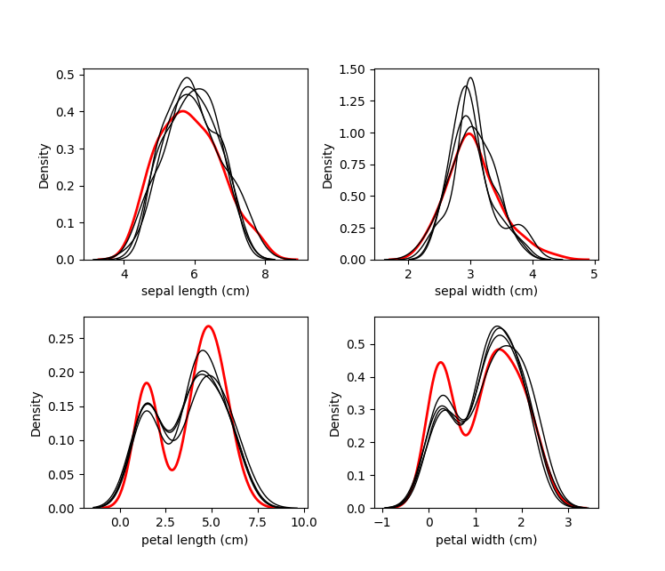 The red line is the original data, and each black line are the imputed
values of each dataset.
### Convergence of Correlation
We are probably interested in knowing how our values between datasets
converged over the iterations. The `plot_correlations` method shows you
a boxplot of the correlations between imputed values in every
combination of datasets, at each iteration. This allows you to see how
correlated the imputations are between datasets, as well as the
convergence over iterations:
``` python
kernel.plot_correlations()
```
The red line is the original data, and each black line are the imputed
values of each dataset.
### Convergence of Correlation
We are probably interested in knowing how our values between datasets
converged over the iterations. The `plot_correlations` method shows you
a boxplot of the correlations between imputed values in every
combination of datasets, at each iteration. This allows you to see how
correlated the imputations are between datasets, as well as the
convergence over iterations:
``` python
kernel.plot_correlations()
```
 ### Variable Importance
We also may be interested in which variables were used to impute each
variable. We can plot this information by using the
`plot_feature_importance` method.
``` python
kernel.plot_feature_importance(dataset=0, annot=True,cmap="YlGnBu",vmin=0, vmax=1)
```
### Variable Importance
We also may be interested in which variables were used to impute each
variable. We can plot this information by using the
`plot_feature_importance` method.
``` python
kernel.plot_feature_importance(dataset=0, annot=True,cmap="YlGnBu",vmin=0, vmax=1)
```
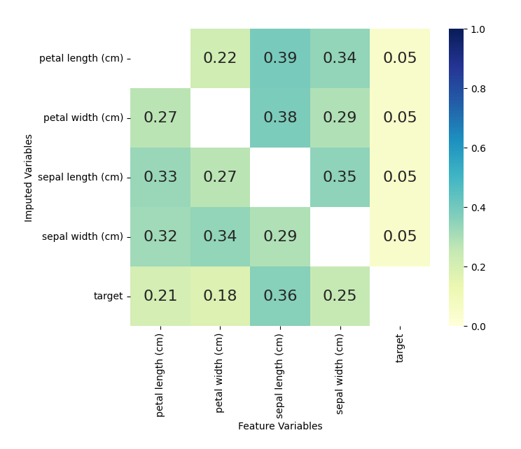 The numbers shown are returned from the
`lightgbm.Booster.feature_importance()` function. Each square represents
the importance of the column variable in imputing the row variable.
### Mean Convergence
If our data is not missing completely at random, we may see that it
takes a few iterations for our models to get the distribution of
imputations right. We can plot the average value of our imputations to
see if this is occurring:
``` python
kernel.plot_mean_convergence(wspace=0.3, hspace=0.4)
```
The numbers shown are returned from the
`lightgbm.Booster.feature_importance()` function. Each square represents
the importance of the column variable in imputing the row variable.
### Mean Convergence
If our data is not missing completely at random, we may see that it
takes a few iterations for our models to get the distribution of
imputations right. We can plot the average value of our imputations to
see if this is occurring:
``` python
kernel.plot_mean_convergence(wspace=0.3, hspace=0.4)
```
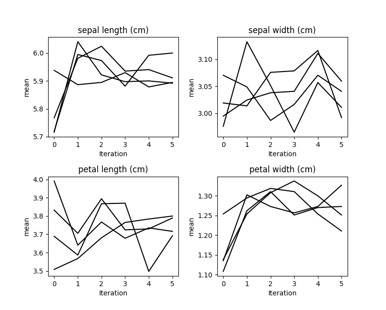 Our data was missing completely at random, so we don’t see any
convergence occurring here.
## Using the Imputed Data
To return the imputed data simply use the `complete_data` method:
``` python
dataset_1 = kernel.complete_data(0)
```
This will return a single specified dataset. Multiple datasets are
typically created so that some measure of confidence around each
prediction can be created.
Since we know what the original data looked like, we can cheat and see
how well the imputations compare to the original data:
``` python
acclist = []
for iteration in range(kernel.iteration_count()+1):
species_na_count = kernel.na_counts[4]
compdat = kernel.complete_data(dataset=0,iteration=iteration)
# Record the accuract of the imputations of species.
acclist.append(
round(1-sum(compdat['species'] != iris['species'])/species_na_count,2)
)
# acclist shows the accuracy of the imputations
# over the iterations.
print(acclist)
```
## [0.35, 0.81, 0.84, 0.84, 0.89, 0.92, 0.89]
In this instance, we went from a low accuracy (what is expected with
random sampling) to a much higher accuracy.
## The MICE Algorithm
Multiple Imputation by Chained Equations ‘fills in’ (imputes) missing
data in a dataset through an iterative series of predictive models. In
each iteration, each specified variable in the dataset is imputed using
the other variables in the dataset. These iterations should be run until
it appears that convergence has been met.
Our data was missing completely at random, so we don’t see any
convergence occurring here.
## Using the Imputed Data
To return the imputed data simply use the `complete_data` method:
``` python
dataset_1 = kernel.complete_data(0)
```
This will return a single specified dataset. Multiple datasets are
typically created so that some measure of confidence around each
prediction can be created.
Since we know what the original data looked like, we can cheat and see
how well the imputations compare to the original data:
``` python
acclist = []
for iteration in range(kernel.iteration_count()+1):
species_na_count = kernel.na_counts[4]
compdat = kernel.complete_data(dataset=0,iteration=iteration)
# Record the accuract of the imputations of species.
acclist.append(
round(1-sum(compdat['species'] != iris['species'])/species_na_count,2)
)
# acclist shows the accuracy of the imputations
# over the iterations.
print(acclist)
```
## [0.35, 0.81, 0.84, 0.84, 0.89, 0.92, 0.89]
In this instance, we went from a low accuracy (what is expected with
random sampling) to a much higher accuracy.
## The MICE Algorithm
Multiple Imputation by Chained Equations ‘fills in’ (imputes) missing
data in a dataset through an iterative series of predictive models. In
each iteration, each specified variable in the dataset is imputed using
the other variables in the dataset. These iterations should be run until
it appears that convergence has been met.
 This process is continued until all specified variables have been
imputed. Additional iterations can be run if it appears that the average
imputed values have not converged, although no more than 5 iterations
are usually necessary.
### Common Use Cases
##### **Data Leakage:**
MICE is particularly useful if missing values are associated with the
target variable in a way that introduces leakage. For instance, let’s
say you wanted to model customer retention at the time of sign up. A
certain variable is collected at sign up or 1 month after sign up. The
absence of that variable is a data leak, since it tells you that the
customer did not retain for 1 month.
##### **Funnel Analysis:**
Information is often collected at different stages of a ‘funnel’. MICE
can be used to make educated guesses about the characteristics of
entities at different points in a funnel.
##### **Confidence Intervals:**
MICE can be used to impute missing values, however it is important to
keep in mind that these imputed values are a prediction. Creating
multiple datasets with different imputed values allows you to do two
types of inference:
- Imputed Value Distribution: A profile can be built for each imputed
value, allowing you to make statements about the likely distribution
of that value.
- Model Prediction Distribution: With multiple datasets, you can build
multiple models and create a distribution of predictions for each
sample. Those samples with imputed values which were not able to be
imputed with much confidence would have a larger variance in their
predictions.
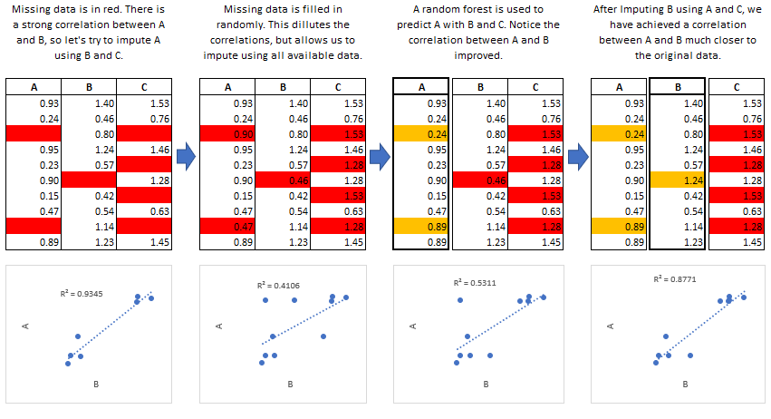
### Predictive Mean Matching
`miceforest` can make use of a procedure called predictive mean matching
(PMM) to select which values are imputed. PMM involves selecting a
datapoint from the original, nonmissing data (candidates) which has a
predicted value close to the predicted value of the missing sample
(bachelors). The closest N (`mean_match_candidates` parameter) values
are selected, from which a value is chosen at random. This can be
specified on a column-by-column basis. Going into more detail from our
example above, we see how this works in practice:
This process is continued until all specified variables have been
imputed. Additional iterations can be run if it appears that the average
imputed values have not converged, although no more than 5 iterations
are usually necessary.
### Common Use Cases
##### **Data Leakage:**
MICE is particularly useful if missing values are associated with the
target variable in a way that introduces leakage. For instance, let’s
say you wanted to model customer retention at the time of sign up. A
certain variable is collected at sign up or 1 month after sign up. The
absence of that variable is a data leak, since it tells you that the
customer did not retain for 1 month.
##### **Funnel Analysis:**
Information is often collected at different stages of a ‘funnel’. MICE
can be used to make educated guesses about the characteristics of
entities at different points in a funnel.
##### **Confidence Intervals:**
MICE can be used to impute missing values, however it is important to
keep in mind that these imputed values are a prediction. Creating
multiple datasets with different imputed values allows you to do two
types of inference:
- Imputed Value Distribution: A profile can be built for each imputed
value, allowing you to make statements about the likely distribution
of that value.
- Model Prediction Distribution: With multiple datasets, you can build
multiple models and create a distribution of predictions for each
sample. Those samples with imputed values which were not able to be
imputed with much confidence would have a larger variance in their
predictions.
### Predictive Mean Matching
`miceforest` can make use of a procedure called predictive mean matching
(PMM) to select which values are imputed. PMM involves selecting a
datapoint from the original, nonmissing data (candidates) which has a
predicted value close to the predicted value of the missing sample
(bachelors). The closest N (`mean_match_candidates` parameter) values
are selected, from which a value is chosen at random. This can be
specified on a column-by-column basis. Going into more detail from our
example above, we see how this works in practice:
 This method is very useful if you have a variable which needs imputing
which has any of the following characteristics:
- Multimodal
- Integer
- Skewed
### Effects of Mean Matching
As an example, let’s construct a dataset with some of the above
characteristics:
``` python
randst = np.random.RandomState(1991)
# random uniform variable
nrws = 1000
uniform_vec = randst.uniform(size=nrws)
def make_bimodal(mean1,mean2,size):
bimodal_1 = randst.normal(size=nrws, loc=mean1)
bimodal_2 = randst.normal(size=nrws, loc=mean2)
bimdvec = []
for i in range(size):
bimdvec.append(randst.choice([bimodal_1[i], bimodal_2[i]]))
return np.array(bimdvec)
# Make 2 Bimodal Variables
close_bimodal_vec = make_bimodal(2,-2,nrws)
far_bimodal_vec = make_bimodal(3,-3,nrws)
# Highly skewed variable correlated with Uniform_Variable
skewed_vec = np.exp(uniform_vec*randst.uniform(size=nrws)*3) + randst.uniform(size=nrws)*3
# Integer variable correlated with Close_Bimodal_Variable and Uniform_Variable
integer_vec = np.round(uniform_vec + close_bimodal_vec/3 + randst.uniform(size=nrws)*2)
# Make a DataFrame
dat = pd.DataFrame(
{
'uniform_var':uniform_vec,
'close_bimodal_var':close_bimodal_vec,
'far_bimodal_var':far_bimodal_vec,
'skewed_var':skewed_vec,
'integer_var':integer_vec
}
)
# Ampute the data.
ampdat = mf.ampute_data(dat,perc=0.25,random_state=randst)
# Plot the original data
import seaborn as sns
import matplotlib.pyplot as plt
g = sns.PairGrid(dat)
g.map(plt.scatter,s=5)
```
This method is very useful if you have a variable which needs imputing
which has any of the following characteristics:
- Multimodal
- Integer
- Skewed
### Effects of Mean Matching
As an example, let’s construct a dataset with some of the above
characteristics:
``` python
randst = np.random.RandomState(1991)
# random uniform variable
nrws = 1000
uniform_vec = randst.uniform(size=nrws)
def make_bimodal(mean1,mean2,size):
bimodal_1 = randst.normal(size=nrws, loc=mean1)
bimodal_2 = randst.normal(size=nrws, loc=mean2)
bimdvec = []
for i in range(size):
bimdvec.append(randst.choice([bimodal_1[i], bimodal_2[i]]))
return np.array(bimdvec)
# Make 2 Bimodal Variables
close_bimodal_vec = make_bimodal(2,-2,nrws)
far_bimodal_vec = make_bimodal(3,-3,nrws)
# Highly skewed variable correlated with Uniform_Variable
skewed_vec = np.exp(uniform_vec*randst.uniform(size=nrws)*3) + randst.uniform(size=nrws)*3
# Integer variable correlated with Close_Bimodal_Variable and Uniform_Variable
integer_vec = np.round(uniform_vec + close_bimodal_vec/3 + randst.uniform(size=nrws)*2)
# Make a DataFrame
dat = pd.DataFrame(
{
'uniform_var':uniform_vec,
'close_bimodal_var':close_bimodal_vec,
'far_bimodal_var':far_bimodal_vec,
'skewed_var':skewed_vec,
'integer_var':integer_vec
}
)
# Ampute the data.
ampdat = mf.ampute_data(dat,perc=0.25,random_state=randst)
# Plot the original data
import seaborn as sns
import matplotlib.pyplot as plt
g = sns.PairGrid(dat)
g.map(plt.scatter,s=5)
```
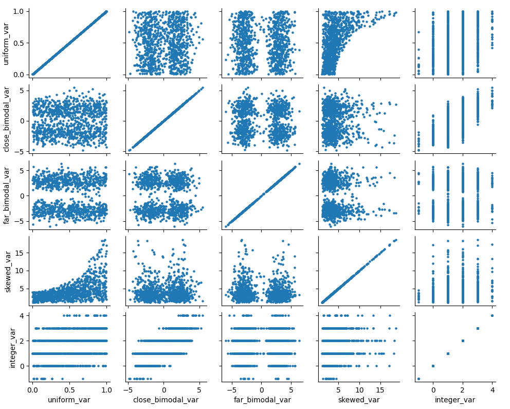 We can see how our variables are distributed and correlated in the graph
above. Now let’s run our imputation process twice, once using mean
matching, and once using the model prediction.
``` python
from miceforest import mean_match_default
scheme_mmc_0 = mean_match_default.copy()
scheme_mmc_5 = mean_match_default.copy()
scheme_mmc_0.set_mean_match_candidates(0)
scheme_mmc_5.set_mean_match_candidates(5)
kernelmeanmatch = mf.ImputationKernel(ampdat, mean_match_scheme=scheme_mmc_5, datasets=1)
kernelmodeloutput = mf.ImputationKernel(ampdat, mean_match_scheme=scheme_mmc_0, datasets=1)
kernelmeanmatch.mice(2)
kernelmodeloutput.mice(2)
```
Let’s look at the effect on the different variables.
##### With Mean Matching
``` python
kernelmeanmatch.plot_imputed_distributions(wspace=0.2,hspace=0.4)
```
We can see how our variables are distributed and correlated in the graph
above. Now let’s run our imputation process twice, once using mean
matching, and once using the model prediction.
``` python
from miceforest import mean_match_default
scheme_mmc_0 = mean_match_default.copy()
scheme_mmc_5 = mean_match_default.copy()
scheme_mmc_0.set_mean_match_candidates(0)
scheme_mmc_5.set_mean_match_candidates(5)
kernelmeanmatch = mf.ImputationKernel(ampdat, mean_match_scheme=scheme_mmc_5, datasets=1)
kernelmodeloutput = mf.ImputationKernel(ampdat, mean_match_scheme=scheme_mmc_0, datasets=1)
kernelmeanmatch.mice(2)
kernelmodeloutput.mice(2)
```
Let’s look at the effect on the different variables.
##### With Mean Matching
``` python
kernelmeanmatch.plot_imputed_distributions(wspace=0.2,hspace=0.4)
```
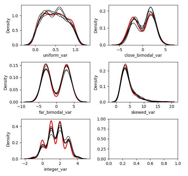 ##### Without Mean Matching
``` python
kernelmodeloutput.plot_imputed_distributions(wspace=0.2,hspace=0.4)
```
##### Without Mean Matching
``` python
kernelmodeloutput.plot_imputed_distributions(wspace=0.2,hspace=0.4)
```
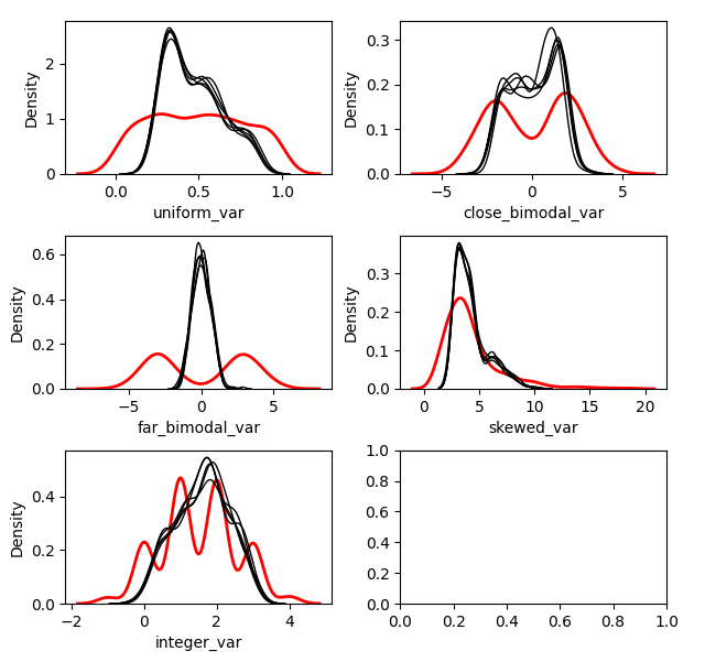 You can see the effects that mean matching has, depending on the
distribution of the data. Simply returning the value from the model
prediction, while it may provide a better ‘fit’, will not provide
imputations with a similair distribution to the original. This may be
beneficial, depending on your goal.
%package -n python3-miceforest
Summary: Missing Value Imputation using LightGBM
Provides: python-miceforest
BuildRequires: python3-devel
BuildRequires: python3-setuptools
BuildRequires: python3-pip
%description -n python3-miceforest
[](https://zenodo.org/badge/latestdoi/289387436)
[](https://pepy.tech/project/miceforest)
[](https://pypi.python.org/pypi/miceforest)
[](https://anaconda.org/conda-forge/miceforest)
[](https://pypi.org/project/miceforest/)
[](https://github.com/AnotherSamWilson/miceforest/actions/workflows/run_tests.yml)
[](https://miceforest.readthedocs.io/en/latest/?badge=latest)
[](https://codecov.io/gh/AnotherSamWilson/miceforest)
## miceforest: Fast, Memory Efficient Imputation with LightGBM
Fast, memory efficient Multiple Imputation by Chained Equations (MICE)
with lightgbm. The R version of this package may be found
[here](https://github.com/FarrellDay/miceRanger).
`miceforest` was designed to be:
- **Fast**
- Uses lightgbm as a backend
- Has efficient mean matching solutions.
- Can utilize GPU training
- **Flexible**
- Can impute pandas dataframes and numpy arrays
- Handles categorical data automatically
- Fits into a sklearn pipeline
- User can customize every aspect of the imputation process
- **Production Ready**
- Can impute new, unseen datasets quickly
- Kernels are efficiently compressed during saving and loading
- Data can be imputed in place to save memory
- Can build models on non-missing data
This document contains a thorough walkthrough of the package,
benchmarks, and an introduction to multiple imputation. More information
on MICE can be found in Stef van Buuren’s excellent online book, which
you can find
[here](https://stefvanbuuren.name/fimd/ch-introduction.html).
#### Table of Contents:
- [Package
Meta](https://github.com/AnotherSamWilson/miceforest#Package-Meta)
- [The
Basics](https://github.com/AnotherSamWilson/miceforest#The-Basics)
- [Basic
Examples](https://github.com/AnotherSamWilson/miceforest#Basic-Examples)
- [Customizing LightGBM
Parameters](https://github.com/AnotherSamWilson/miceforest#Customizing-LightGBM-Parameters)
- [Available Mean Match
Schemes](https://github.com/AnotherSamWilson/miceforest#Controlling-Tree-Growth)
- [Imputing New Data with Existing
Models](https://github.com/AnotherSamWilson/miceforest#Imputing-New-Data-with-Existing-Models)
- [Saving and Loading
Kernels](https://github.com/AnotherSamWilson/miceforest#Saving-and-Loading-Kernels)
- [Implementing sklearn
Pipelines](https://github.com/AnotherSamWilson/miceforest#Implementing-sklearn-Pipelines)
- [Advanced
Features](https://github.com/AnotherSamWilson/miceforest#Advanced-Features)
- [Customizing the Imputation
Process](https://github.com/AnotherSamWilson/miceforest#Customizing-the-Imputation-Process)
- [Building Models on Nonmissing
Data](https://github.com/AnotherSamWilson/miceforest#Building-Models-on-Nonmissing-Data)
- [Tuning
Parameters](https://github.com/AnotherSamWilson/miceforest#Tuning-Parameters)
- [On
Reproducibility](https://github.com/AnotherSamWilson/miceforest#On-Reproducibility)
- [How to Make the Process
Faster](https://github.com/AnotherSamWilson/miceforest#How-to-Make-the-Process-Faster)
- [Imputing Data In
Place](https://github.com/AnotherSamWilson/miceforest#Imputing-Data-In-Place)
- [Diagnostic
Plotting](https://github.com/AnotherSamWilson/miceforest#Diagnostic-Plotting)
- [Imputed
Distributions](https://github.com/AnotherSamWilson/miceforest#Distribution-of-Imputed-Values)
- [Correlation
Convergence](https://github.com/AnotherSamWilson/miceforest#Convergence-of-Correlation)
- [Variable
Importance](https://github.com/AnotherSamWilson/miceforest#Variable-Importance)
- [Mean
Convergence](https://github.com/AnotherSamWilson/miceforest#Variable-Importance)
- [Benchmarks](https://github.com/AnotherSamWilson/miceforest#Benchmarks)
- [Using the Imputed
Data](https://github.com/AnotherSamWilson/miceforest#Using-the-Imputed-Data)
- [The MICE
Algorithm](https://github.com/AnotherSamWilson/miceforest#The-MICE-Algorithm)
- [Introduction](https://github.com/AnotherSamWilson/miceforest#The-MICE-Algorithm)
- [Common Use
Cases](https://github.com/AnotherSamWilson/miceforest#Common-Use-Cases)
- [Predictive Mean
Matching](https://github.com/AnotherSamWilson/miceforest#Predictive-Mean-Matching)
- [Effects of Mean
Matching](https://github.com/AnotherSamWilson/miceforest#Effects-of-Mean-Matching)
## Package Meta
### Installation
This package can be installed using either pip or conda, through
conda-forge:
``` bash
# Using pip
$ pip install miceforest --no-cache-dir
# Using conda
$ conda install -c conda-forge miceforest
```
You can also download the latest development version from this
repository. If you want to install from github with conda, you must
first run `conda install pip git`.
``` bash
$ pip install git+https://github.com/AnotherSamWilson/miceforest.git
```
### Classes
miceforest has 3 main classes which the user will interact with:
- [`ImputationKernel`](https://miceforest.readthedocs.io/en/latest/ik/miceforest.ImputationKernel.html#miceforest.ImputationKernel)
- This class contains the raw data off of which the `mice` algorithm
is performed. During this process, models will be trained, and the
imputed (predicted) values will be stored. These values can be used
to fill in the missing values of the raw data. The raw data can be
copied, or referenced directly. Models can be saved, and used to
impute new datasets.
- [`ImputedData`](https://miceforest.readthedocs.io/en/latest/ik/miceforest.ImputedData.html#miceforest.ImputedData)
- The result of `ImputationKernel.impute_new_data(new_data)`. This
contains the raw data in `new_data` as well as the imputed values.
- [`MeanMatchScheme`](https://miceforest.readthedocs.io/en/latest/ik/miceforest.MeanMatchScheme.html#miceforest.MeanMatchScheme)
- Determines how mean matching should be carried out. There are 3
built-in mean match schemes available in miceforest, discussed
below.
## The Basics
We will be looking at a few simple examples of imputation. We need to
load the packages, and define the data:
``` python
import miceforest as mf
from sklearn.datasets import load_iris
import pandas as pd
import numpy as np
# Load data and introduce missing values
iris = pd.concat(load_iris(as_frame=True,return_X_y=True),axis=1)
iris.rename({"target": "species"}, inplace=True, axis=1)
iris['species'] = iris['species'].astype('category')
iris_amp = mf.ampute_data(iris,perc=0.25,random_state=1991)
```
### Basic Examples
If you only want to create a single imputed dataset, you can use
[`ImputationKernel`](https://miceforest.readthedocs.io/en/latest/ik/miceforest.ImputationKernel.html#miceforest.ImputationKernel)
with some default settings:
``` python
# Create kernel.
kds = mf.ImputationKernel(
iris_amp,
save_all_iterations=True,
random_state=1991
)
# Run the MICE algorithm for 2 iterations
kds.mice(2)
# Return the completed dataset.
iris_complete = kds.complete_data()
```
There are also an array of plotting functions available, these are
discussed below in the section [Diagnostic
Plotting](https://github.com/AnotherSamWilson/miceforest#Diagnostic-Plotting).
We usually don’t want to impute just a single dataset. In statistics,
multiple imputation is a process by which the uncertainty/other effects
caused by missing values can be examined by creating multiple different
imputed datasets.
[`ImputationKernel`](https://miceforest.readthedocs.io/en/latest/ik/miceforest.ImputationKernel.html#miceforest.ImputationKernel)
can contain an arbitrary number of different datasets, all of which have
gone through mutually exclusive imputation processes:
``` python
# Create kernel.
kernel = mf.ImputationKernel(
iris_amp,
datasets=4,
save_all_iterations=True,
random_state=1
)
# Run the MICE algorithm for 2 iterations on each of the datasets
kernel.mice(2)
# Printing the kernel will show you some high level information.
print(kernel)
```
##
## Class: ImputationKernel
## Datasets: 4
## Iterations: 2
## Data Samples: 150
## Data Columns: 5
## Imputed Variables: 5
## save_all_iterations: True
After we have run mice, we can obtain our completed dataset directly
from the kernel:
``` python
completed_dataset = kernel.complete_data(dataset=2)
print(completed_dataset.isnull().sum(0))
```
## sepal length (cm) 0
## sepal width (cm) 0
## petal length (cm) 0
## petal width (cm) 0
## species 0
## dtype: int64
### Customizing LightGBM Parameters
Parameters can be passed directly to lightgbm in several different ways.
Parameters you wish to apply globally to every model can simply be
passed as kwargs to `mice`:
``` python
# Run the MICE algorithm for 1 more iteration on the kernel with new parameters
kernel.mice(iterations=1,n_estimators=50)
```
You can also pass pass variable-specific arguments to
`variable_parameters` in mice. For instance, let’s say you noticed the
imputation of the `[species]` column was taking a little longer, because
it is multiclass. You could decrease the n\_estimators specifically for
that column with:
``` python
# Run the MICE algorithm for 2 more iterations on the kernel
kernel.mice(
iterations=1,
variable_parameters={'species': {'n_estimators': 25}},
n_estimators=50
)
# Let's get the actual models for these variables:
species_model = kernel.get_model(dataset=0,variable="species")
sepalwidth_model = kernel.get_model(dataset=0,variable="sepal width (cm)")
print(
f"""Species used {str(species_model.params["num_iterations"])} iterations
Sepal Width used {str(sepalwidth_model.params["num_iterations"])} iterations
"""
)
```
## Species used 25 iterations
## Sepal Width used 50 iterations
In this scenario, any parameters specified in `variable_parameters`
takes presidence over the kwargs.
Since we can pass any parameters we want to LightGBM, we can completely
customize how our models are built. That includes how the data should be
modeled. If your data contains count data, or any other data which can
be parameterized by lightgbm, you can simply specify that variable to be
modeled with the corresponding objective function.
For example, let’s pretend `sepal width (cm)` is a count field which can
be parameterized by a Poisson distribution. Let’s also change our
boosting method to gradient boosted trees:
``` python
# Create kernel.
cust_kernel = mf.ImputationKernel(
iris_amp,
datasets=1,
random_state=1
)
cust_kernel.mice(
iterations=1,
variable_parameters={'sepal width (cm)': {'objective': 'poisson'}},
boosting = 'gbdt',
min_sum_hessian_in_leaf=0.01
)
```
Other nice parameters like `monotone_constraints` can also be passed.
Setting the parameter `device: 'gpu'` will utilize GPU learning, if
LightGBM is set up to do this on your machine.
### Available Mean Match Schemes
Note: It is probably a good idea to read [this
section](https://github.com/AnotherSamWilson/miceforest#Predictive-Mean-Matching)
first, to get some context on how mean matching works.
The class `miceforest.MeanMatchScheme` contains information about how
mean matching should be performed, such as:
1) Mean matching functions
2) Mean matching candidates
3) How to get predictions from a lightgbm model
4) The datatypes predictions are stored as
There are three pre-built mean matching schemes that come with
`miceforest`:
``` python
from miceforest import (
mean_match_default,
mean_match_fast_cat,
mean_match_shap
)
# To get information for each, use help()
# help(mean_match_default)
```
These schemes mostly differ in their strategy for performing mean
matching
- **mean\_match\_default** - medium speed, medium imputation quality
- Categorical: perform a K Nearest Neighbors search on the
candidate class probabilities, where K = mmc. Select 1 at
random, and choose the associated candidate value as the
imputation value.
- Numeric: Perform a K Nearest Neighbors search on the candidate
predictions, where K = mmc. Select 1 at random, and choose the
associated candidate value as the imputation value.
- **mean\_match\_fast\_cat** - fastest speed, lowest imputation
quality
- Categorical: return class based on random draw weighted by class
probability for each sample.
- Numeric: perform a K Nearest Neighbors search on the candidate
class probabilities, where K = mmc. Select 1 at random, and
choose the associated candidate value as the imputation value.
- **mean\_match\_shap** - slowest speed, highest imputation quality
for large datasets
- Categorical: perform a K Nearest Neighbors search on the
candidate prediction shap values, where K = mmc. Select 1 at
random, and choose the associated candidate value as the
imputation value.
- Numeric: perform a K Nearest Neighbors search on the candidate
prediction shap values, where K = mmc. Select 1 at random, and
choose the associated candidate value as the imputation value.
As a special case, if the mean\_match\_candidates is set to 0, the
following behavior is observed for all schemes:
- Categorical: the class with the highest probability is chosen.
- Numeric: the predicted value is used
These mean matching schemes can be updated and customized, we show an
example below in the advanced section.
### Imputing New Data with Existing Models
Multiple Imputation can take a long time. If you wish to impute a
dataset using the MICE algorithm, but don’t have time to train new
models, it is possible to impute new datasets using a `ImputationKernel`
object. The `impute_new_data()` function uses the models collected by
`ImputationKernel` to perform multiple imputation without updating the
models at each iteration:
``` python
# Our 'new data' is just the first 15 rows of iris_amp
from datetime import datetime
# Define our new data as the first 15 rows
new_data = iris_amp.iloc[range(15)]
# Imputing new data can often be made faster by
# first compiling candidate predictions
kernel.compile_candidate_preds()
start_t = datetime.now()
new_data_imputed = kernel.impute_new_data(new_data=new_data)
print(f"New Data imputed in {(datetime.now() - start_t).total_seconds()} seconds")
```
## New Data imputed in 0.507115 seconds
All of the imputation parameters (variable\_schema,
mean\_match\_candidates, etc) will be carried over from the original
`ImputationKernel` object. When mean matching, the candidate values are
pulled from the original kernel dataset. To impute new data, the
`save_models` parameter in `ImputationKernel` must be \> 0. If
`save_models == 1`, the model from the latest iteration is saved for
each variable. If `save_models > 1`, the model from each iteration is
saved. This allows for new data to be imputed in a more similar fashion
to the original mice procedure.
### Saving and Loading Kernels
Kernels can be saved using the `.save_kernel()` method, and then loaded
again using the `utils.load_kernel()` function. Internally, this
procedure uses `blosc` and `dill` packages to do the following:
1. Convert working data to parquet bytes (if it is a pandas dataframe)
2. Serialize the kernel
3. Compress this serialization
4. Save to a file
### Implementing sklearn Pipelines
kernels can be fit into sklearn pipelines to impute training and scoring
datasets:
``` python
import numpy as np
from sklearn.preprocessing import StandardScaler
from sklearn.datasets import make_classification
from sklearn.model_selection import train_test_split
from sklearn.pipeline import Pipeline
import miceforest as mf
# Define our data
X, y = make_classification(random_state=0)
# Ampute and split the training data
X = mf.utils.ampute_data(X)
X_train, X_test, y_train, y_test = train_test_split(X, y, random_state=0)
# Initialize our miceforest kernel. datasets parameter should be 1,
# we don't want to return multiple datasets.
pipe_kernel = mf.ImputationKernel(X_train, datasets=1)
# Define our pipeline
pipe = Pipeline([
('impute', pipe_kernel),
('scaler', StandardScaler()),
])
# Fit on and transform our training data.
# Only use 2 iterations of mice.
X_train_t = pipe.fit_transform(
X_train,
y_train,
impute__iterations=2
)
# Transform the test data as well
X_test_t = pipe.transform(X_test)
# Show that neither now have missing values.
assert not np.any(np.isnan(X_train_t))
assert not np.any(np.isnan(X_test_t))
```
## Advanced Features
Multiple imputation is a complex process. However, `miceforest` allows
all of the major components to be switched out and customized by the
user.
### Customizing the Imputation Process
It is possible to heavily customize our imputation procedure by
variable. By passing a named list to `variable_schema`, you can specify
the predictor variables for each imputed variable. You can also specify
`mean_match_candidates` and `data_subset` by variable by passing a dict
of valid values, with variable names as keys. You can even replace the
entire default mean matching function for certain objectives if desired.
Below is an *extremely* convoluted setup, which you would probably never
want to use. It simply shows what is possible:
``` python
# Use the default mean match schema as our base
from miceforest import mean_match_default
mean_match_custom = mean_match_default.copy()
# Define a mean matching function that
# just randomly shuffles the predictions
def custom_mmf(bachelor_preds):
np.random.shuffle(bachelor_preds)
return bachelor_preds
# Specify that our custom function should be
# used to perform mean matching on any variable
# that was modeled with a poisson objective:
mean_match_custom.set_mean_match_function(
{"poisson": custom_mmf}
)
# Set the mean match candidates by variable
mean_match_custom.set_mean_match_candidates(
{
'sepal width (cm)': 3,
'petal width (cm)': 0
}
)
# Define which variables should be used to model others
variable_schema = {
'sepal width (cm)': ['species','petal width (cm)'],
'petal width (cm)': ['species','sepal length (cm)']
}
# Subset the candidate data to 50 rows for sepal width (cm).
variable_subset = {
'sepal width (cm)': 50
}
# Specify that petal width (cm) should be modeled by the
# poisson objective. Our custom mean matching function
# above will be used for this variable.
variable_parameters = {
'petal width (cm)': {"objective": "poisson"}
}
cust_kernel = mf.ImputationKernel(
iris_amp,
datasets=3,
mean_match_scheme=mean_match_custom,
variable_schema=variable_schema,
data_subset=variable_subset
)
cust_kernel.mice(iterations=1, variable_parameters=variable_parameters)
```
The mean matching function can take any number of the following
arguments. If a function does not take one of these arguments, then the
process will not prepare that data for mean matching.
``` python
from miceforest.MeanMatchScheme import AVAILABLE_MEAN_MATCH_ARGS
print("\n".join(AVAILABLE_MEAN_MATCH_ARGS))
```
## mean_match_candidates
## lgb_booster
## bachelor_preds
## bachelor_features
## candidate_values
## candidate_features
## candidate_preds
## random_state
## hashed_seeds
### Building Models on Nonmissing Data
The MICE process itself is used to impute missing data in a dataset.
However, sometimes a variable can be fully recognized in the training
data, but needs to be imputed later on in a different dataset. It is
possible to train models to impute variables even if they have no
missing values by setting `train_nonmissing=True`. In this case,
`variable_schema` is treated as the list of variables to train models
on. `imputation_order` only affects which variables actually have their
values imputed, it does not affect which variables have models trained:
``` python
orig_missing_cols = ["sepal length (cm)", "sepal width (cm)"]
new_missing_cols = ["sepal length (cm)", "sepal width (cm)", "species"]
# Training data only contains 2 columns with missing data
iris_amp2 = iris.copy()
iris_amp2[orig_missing_cols] = mf.ampute_data(
iris_amp2[orig_missing_cols],
perc=0.25,
random_state=1991
)
# Specify that models should also be trained for species column
var_sch = new_missing_cols
cust_kernel = mf.ImputationKernel(
iris_amp2,
datasets=1,
variable_schema=var_sch,
train_nonmissing=True
)
cust_kernel.mice(1)
# New data has missing values in species column
iris_amp2_new = iris.iloc[range(10),:].copy()
iris_amp2_new[new_missing_cols] = mf.ampute_data(
iris_amp2_new[new_missing_cols],
perc=0.25,
random_state=1991
)
# Species column can still be imputed
iris_amp2_new_imp = cust_kernel.impute_new_data(iris_amp2_new)
iris_amp2_new_imp.complete_data(0).isnull().sum()
```
## sepal length (cm) 0
## sepal width (cm) 0
## petal length (cm) 0
## petal width (cm) 0
## species 0
## dtype: int64
Here, we knew that the species column in our new data would need to be
imputed. Therefore, we specified that a model should be built for all 3
variables in the `variable_schema` (passing a dict of target - feature
pairs would also have worked).
### Tuning Parameters
`miceforest` allows you to tune the parameters on a kernel dataset.
These parameters can then be used to build the models in future
iterations of mice. In its most simple invocation, you can just call the
function with the desired optimization steps:
``` python
# Using the first ImputationKernel in kernel to tune parameters
# with the default settings.
optimal_parameters, losses = kernel.tune_parameters(
dataset=0,
optimization_steps=5
)
# Run mice with our newly tuned parameters.
kernel.mice(1, variable_parameters=optimal_parameters)
# The optimal parameters are kept in ImputationKernel.optimal_parameters:
print(optimal_parameters)
```
## {0: {'boosting': 'gbdt', 'num_iterations': 165, 'max_depth': 8, 'num_leaves': 20, 'min_data_in_leaf': 1, 'min_sum_hessian_in_leaf': 0.1, 'min_gain_to_split': 0.0, 'bagging_fraction': 0.2498838792503861, 'feature_fraction': 1.0, 'feature_fraction_bynode': 0.6020460898858531, 'bagging_freq': 1, 'verbosity': -1, 'objective': 'regression', 'learning_rate': 0.02, 'cat_smooth': 17.807024990062555}, 1: {'boosting': 'gbdt', 'num_iterations': 94, 'max_depth': 8, 'num_leaves': 14, 'min_data_in_leaf': 4, 'min_sum_hessian_in_leaf': 0.1, 'min_gain_to_split': 0.0, 'bagging_fraction': 0.7802435334180599, 'feature_fraction': 1.0, 'feature_fraction_bynode': 0.6856668707631843, 'bagging_freq': 1, 'verbosity': -1, 'objective': 'regression', 'learning_rate': 0.02, 'cat_smooth': 4.802568893662679}, 2: {'boosting': 'gbdt', 'num_iterations': 229, 'max_depth': 8, 'num_leaves': 4, 'min_data_in_leaf': 8, 'min_sum_hessian_in_leaf': 0.1, 'min_gain_to_split': 0.0, 'bagging_fraction': 0.9565982004313843, 'feature_fraction': 1.0, 'feature_fraction_bynode': 0.6065024947204825, 'bagging_freq': 1, 'verbosity': -1, 'objective': 'regression', 'learning_rate': 0.02, 'cat_smooth': 17.2138799939537}, 3: {'boosting': 'gbdt', 'num_iterations': 182, 'max_depth': 8, 'num_leaves': 20, 'min_data_in_leaf': 4, 'min_sum_hessian_in_leaf': 0.1, 'min_gain_to_split': 0.0, 'bagging_fraction': 0.7251674145835884, 'feature_fraction': 1.0, 'feature_fraction_bynode': 0.9262368919526676, 'bagging_freq': 1, 'verbosity': -1, 'objective': 'regression', 'learning_rate': 0.02, 'cat_smooth': 5.780326477879999}, 4: {'boosting': 'gbdt', 'num_iterations': 208, 'max_depth': 8, 'num_leaves': 4, 'min_data_in_leaf': 7, 'min_sum_hessian_in_leaf': 0.1, 'min_gain_to_split': 0.0, 'bagging_fraction': 0.6746301598613926, 'feature_fraction': 1.0, 'feature_fraction_bynode': 0.20999114041328495, 'bagging_freq': 1, 'verbosity': -1, 'objective': 'multiclass', 'num_class': 3, 'learning_rate': 0.02, 'cat_smooth': 8.604908973256704}}
This will perform 10 fold cross validation on random samples of
parameters. By default, all variables models are tuned. If you are
curious about the default parameter space that is searched within, check
out the `miceforest.default_lightgbm_parameters` module.
The parameter tuning is pretty flexible. If you wish to set some model
parameters static, or to change the bounds that are searched in, you can
simply pass this information to either the `variable_parameters`
parameter, `**kwbounds`, or both:
``` python
# Using a complicated setup:
optimal_parameters, losses = kernel.tune_parameters(
dataset=0,
variables = ['sepal width (cm)','species','petal width (cm)'],
variable_parameters = {
'sepal width (cm)': {'bagging_fraction': 0.5},
'species': {'bagging_freq': (5,10)}
},
optimization_steps=5,
extra_trees = [True, False]
)
kernel.mice(1, variable_parameters=optimal_parameters)
```
In this example, we did a few things - we specified that only `sepal
width (cm)`, `species`, and `petal width (cm)` should be tuned. We also
specified some specific parameters in `variable_parameters.` Notice that
`bagging_fraction` was passed as a scalar, `0.5`. This means that, for
the variable `sepal width (cm)`, the parameter `bagging_fraction` will
be set as that number and not be tuned. We did the opposite for
`bagging_freq`. We specified bounds that the process should search in.
We also passed the argument `extra_trees` as a list. Since it was passed
to \*\*kwbounds, this parameter will apply to all variables that are
being tuned. Passing values as a list tells the process that it should
randomly sample values from the list, instead of treating them as set of
counts to search within.
The tuning process follows these rules for different parameter values it
finds:
- Scalar: That value is used, and not tuned.
- Tuple: Should be length 2. Treated as the lower and upper bound to
search in.
- List: Treated as a distinct list of values to try randomly.
### On Reproducibility
`miceforest` allows for different “levels” of reproducibility, global
and record-level.
##### **Global Reproducibility**
Global reproducibility ensures that the same values will be imputed if
the same code is run multiple times. To ensure global reproducibility,
all the user needs to do is set a `random_state` when the kernel is
initialized.
##### **Record-Level Reproducibility**
Sometimes we want to obtain reproducible imputations at the record
level, without having to pass the same dataset. This is possible by
passing a list of record-specific seeds to the `random_seed_array`
parameter. This is useful if imputing new data multiple times, and you
would like imputations for each row to match each time it is imputed.
``` python
# Define seeds for the data, and impute iris
random_seed_array = np.random.randint(9999, size=150)
iris_imputed = kernel.impute_new_data(
iris_amp,
random_state=4,
random_seed_array=random_seed_array
)
# Select a random sample
new_inds = np.random.choice(150, size=15)
new_data = iris_amp.loc[new_inds]
new_seeds = random_seed_array[new_inds]
new_imputed = kernel.impute_new_data(
new_data,
random_state=4,
random_seed_array=new_seeds
)
# We imputed the same values for the 15 values each time,
# because each record was associated with the same seed.
assert new_imputed.complete_data(0).equals(iris_imputed.complete_data(0).loc[new_inds])
```
Note that record-level reproducibility is only possible in the
`impute_new_data` function, there are no guarantees of record-level
reproducibility in imputations between the kernel and new data.
### How to Make the Process Faster
Multiple Imputation is one of the most robust ways to handle missing
data - but it can take a long time. There are several strategies you can
use to decrease the time a process takes to run:
- Decrease `data_subset`. By default all non-missing datapoints for
each variable are used to train the model and perform mean matching.
This can cause the model training nearest-neighbors search to take a
long time for large data. A subset of these points can be searched
instead by using `data_subset`.
- If categorical columns are taking a long time, you can use the
`mean_match_fast_cat` scheme. You can also set different parameters
specifically for categorical columns, like smaller
`bagging_fraction` or `num_iterations`.
- If you need to impute new data faster, compile the predictions with
the `compile_candidate_preds` method. This stores the predictions
for each model, so it does not need to be re-calculated at each
iteration.
- Convert your data to a numpy array. Numpy arrays are much faster to
index. While indexing overhead is avoided as much as possible, there
is no getting around it. Consider comverting to `float32` datatype
as well, as it will cause the resulting object to take up much less
memory.
- Decrease `mean_match_candidates`. The maximum number of neighbors
that are considered with the default parameters is 10. However, for
large datasets, this can still be an expensive operation. Consider
explicitly setting `mean_match_candidates` lower.
- Use different lightgbm parameters. lightgbm is usually not the
problem, however if a certain variable has a large number of
classes, then the max number of trees actually grown is (\# classes)
\* (n\_estimators). You can specifically decrease the bagging
fraction or n\_estimators for large multi-class variables, or grow
less trees in general.
- Use a faster mean matching function. The default mean matching
function uses the scipy.Spatial.KDtree algorithm. There are faster
alternatives out there, if you think mean matching is the holdup.
### Imputing Data In Place
It is possible to run the entire process without copying the dataset. If
`copy_data=False`, then the data is referenced directly:
``` python
kernel_inplace = mf.ImputationKernel(
iris_amp,
datasets=1,
copy_data=False
)
kernel_inplace.mice(2)
```
Note, that this probably won’t (but could) change the original dataset
in undesirable ways. Throughout the `mice` procedure, imputed values are
stored directly in the original data. At the end, the missing values are
put back as `np.NaN`.
We can also complete our original data in place:
``` python
kernel_inplace.complete_data(dataset=0, inplace=True)
print(iris_amp.isnull().sum(0))
```
## sepal length (cm) 0
## sepal width (cm) 0
## petal length (cm) 0
## petal width (cm) 0
## species 0
## dtype: int64
This is useful if the dataset is large, and copies can’t be made in
memory.
## Diagnostic Plotting
As of now, miceforest has four diagnostic plots available.
### Distribution of Imputed-Values
We probably want to know how the imputed values are distributed. We can
plot the original distribution beside the imputed distributions in each
dataset by using the `plot_imputed_distributions` method of an
`ImputationKernel` object:
``` python
kernel.plot_imputed_distributions(wspace=0.3,hspace=0.3)
```
The red line is the original data, and each black line are the imputed
values of each dataset.
### Convergence of Correlation
We are probably interested in knowing how our values between datasets
converged over the iterations. The `plot_correlations` method shows you
a boxplot of the correlations between imputed values in every
combination of datasets, at each iteration. This allows you to see how
correlated the imputations are between datasets, as well as the
convergence over iterations:
``` python
kernel.plot_correlations()
```
### Variable Importance
We also may be interested in which variables were used to impute each
variable. We can plot this information by using the
`plot_feature_importance` method.
``` python
kernel.plot_feature_importance(dataset=0, annot=True,cmap="YlGnBu",vmin=0, vmax=1)
```
The numbers shown are returned from the
`lightgbm.Booster.feature_importance()` function. Each square represents
the importance of the column variable in imputing the row variable.
### Mean Convergence
If our data is not missing completely at random, we may see that it
takes a few iterations for our models to get the distribution of
imputations right. We can plot the average value of our imputations to
see if this is occurring:
``` python
kernel.plot_mean_convergence(wspace=0.3, hspace=0.4)
```
Our data was missing completely at random, so we don’t see any
convergence occurring here.
## Using the Imputed Data
To return the imputed data simply use the `complete_data` method:
``` python
dataset_1 = kernel.complete_data(0)
```
This will return a single specified dataset. Multiple datasets are
typically created so that some measure of confidence around each
prediction can be created.
Since we know what the original data looked like, we can cheat and see
how well the imputations compare to the original data:
``` python
acclist = []
for iteration in range(kernel.iteration_count()+1):
species_na_count = kernel.na_counts[4]
compdat = kernel.complete_data(dataset=0,iteration=iteration)
# Record the accuract of the imputations of species.
acclist.append(
round(1-sum(compdat['species'] != iris['species'])/species_na_count,2)
)
# acclist shows the accuracy of the imputations
# over the iterations.
print(acclist)
```
## [0.35, 0.81, 0.84, 0.84, 0.89, 0.92, 0.89]
In this instance, we went from a low accuracy (what is expected with
random sampling) to a much higher accuracy.
## The MICE Algorithm
Multiple Imputation by Chained Equations ‘fills in’ (imputes) missing
data in a dataset through an iterative series of predictive models. In
each iteration, each specified variable in the dataset is imputed using
the other variables in the dataset. These iterations should be run until
it appears that convergence has been met.
This process is continued until all specified variables have been
imputed. Additional iterations can be run if it appears that the average
imputed values have not converged, although no more than 5 iterations
are usually necessary.
### Common Use Cases
##### **Data Leakage:**
MICE is particularly useful if missing values are associated with the
target variable in a way that introduces leakage. For instance, let’s
say you wanted to model customer retention at the time of sign up. A
certain variable is collected at sign up or 1 month after sign up. The
absence of that variable is a data leak, since it tells you that the
customer did not retain for 1 month.
##### **Funnel Analysis:**
Information is often collected at different stages of a ‘funnel’. MICE
can be used to make educated guesses about the characteristics of
entities at different points in a funnel.
##### **Confidence Intervals:**
MICE can be used to impute missing values, however it is important to
keep in mind that these imputed values are a prediction. Creating
multiple datasets with different imputed values allows you to do two
types of inference:
- Imputed Value Distribution: A profile can be built for each imputed
value, allowing you to make statements about the likely distribution
of that value.
- Model Prediction Distribution: With multiple datasets, you can build
multiple models and create a distribution of predictions for each
sample. Those samples with imputed values which were not able to be
imputed with much confidence would have a larger variance in their
predictions.
### Predictive Mean Matching
`miceforest` can make use of a procedure called predictive mean matching
(PMM) to select which values are imputed. PMM involves selecting a
datapoint from the original, nonmissing data (candidates) which has a
predicted value close to the predicted value of the missing sample
(bachelors). The closest N (`mean_match_candidates` parameter) values
are selected, from which a value is chosen at random. This can be
specified on a column-by-column basis. Going into more detail from our
example above, we see how this works in practice:
This method is very useful if you have a variable which needs imputing
which has any of the following characteristics:
- Multimodal
- Integer
- Skewed
### Effects of Mean Matching
As an example, let’s construct a dataset with some of the above
characteristics:
``` python
randst = np.random.RandomState(1991)
# random uniform variable
nrws = 1000
uniform_vec = randst.uniform(size=nrws)
def make_bimodal(mean1,mean2,size):
bimodal_1 = randst.normal(size=nrws, loc=mean1)
bimodal_2 = randst.normal(size=nrws, loc=mean2)
bimdvec = []
for i in range(size):
bimdvec.append(randst.choice([bimodal_1[i], bimodal_2[i]]))
return np.array(bimdvec)
# Make 2 Bimodal Variables
close_bimodal_vec = make_bimodal(2,-2,nrws)
far_bimodal_vec = make_bimodal(3,-3,nrws)
# Highly skewed variable correlated with Uniform_Variable
skewed_vec = np.exp(uniform_vec*randst.uniform(size=nrws)*3) + randst.uniform(size=nrws)*3
# Integer variable correlated with Close_Bimodal_Variable and Uniform_Variable
integer_vec = np.round(uniform_vec + close_bimodal_vec/3 + randst.uniform(size=nrws)*2)
# Make a DataFrame
dat = pd.DataFrame(
{
'uniform_var':uniform_vec,
'close_bimodal_var':close_bimodal_vec,
'far_bimodal_var':far_bimodal_vec,
'skewed_var':skewed_vec,
'integer_var':integer_vec
}
)
# Ampute the data.
ampdat = mf.ampute_data(dat,perc=0.25,random_state=randst)
# Plot the original data
import seaborn as sns
import matplotlib.pyplot as plt
g = sns.PairGrid(dat)
g.map(plt.scatter,s=5)
```
We can see how our variables are distributed and correlated in the graph
above. Now let’s run our imputation process twice, once using mean
matching, and once using the model prediction.
``` python
from miceforest import mean_match_default
scheme_mmc_0 = mean_match_default.copy()
scheme_mmc_5 = mean_match_default.copy()
scheme_mmc_0.set_mean_match_candidates(0)
scheme_mmc_5.set_mean_match_candidates(5)
kernelmeanmatch = mf.ImputationKernel(ampdat, mean_match_scheme=scheme_mmc_5, datasets=1)
kernelmodeloutput = mf.ImputationKernel(ampdat, mean_match_scheme=scheme_mmc_0, datasets=1)
kernelmeanmatch.mice(2)
kernelmodeloutput.mice(2)
```
Let’s look at the effect on the different variables.
##### With Mean Matching
``` python
kernelmeanmatch.plot_imputed_distributions(wspace=0.2,hspace=0.4)
```
##### Without Mean Matching
``` python
kernelmodeloutput.plot_imputed_distributions(wspace=0.2,hspace=0.4)
```
You can see the effects that mean matching has, depending on the
distribution of the data. Simply returning the value from the model
prediction, while it may provide a better ‘fit’, will not provide
imputations with a similair distribution to the original. This may be
beneficial, depending on your goal.
%package help
Summary: Development documents and examples for miceforest
Provides: python3-miceforest-doc
%description help
[](https://zenodo.org/badge/latestdoi/289387436)
[](https://pepy.tech/project/miceforest)
[](https://pypi.python.org/pypi/miceforest)
[](https://anaconda.org/conda-forge/miceforest)
[](https://pypi.org/project/miceforest/)
[](https://github.com/AnotherSamWilson/miceforest/actions/workflows/run_tests.yml)
[](https://miceforest.readthedocs.io/en/latest/?badge=latest)
[](https://codecov.io/gh/AnotherSamWilson/miceforest)
## miceforest: Fast, Memory Efficient Imputation with LightGBM
Fast, memory efficient Multiple Imputation by Chained Equations (MICE)
with lightgbm. The R version of this package may be found
[here](https://github.com/FarrellDay/miceRanger).
`miceforest` was designed to be:
- **Fast**
- Uses lightgbm as a backend
- Has efficient mean matching solutions.
- Can utilize GPU training
- **Flexible**
- Can impute pandas dataframes and numpy arrays
- Handles categorical data automatically
- Fits into a sklearn pipeline
- User can customize every aspect of the imputation process
- **Production Ready**
- Can impute new, unseen datasets quickly
- Kernels are efficiently compressed during saving and loading
- Data can be imputed in place to save memory
- Can build models on non-missing data
This document contains a thorough walkthrough of the package,
benchmarks, and an introduction to multiple imputation. More information
on MICE can be found in Stef van Buuren’s excellent online book, which
you can find
[here](https://stefvanbuuren.name/fimd/ch-introduction.html).
#### Table of Contents:
- [Package
Meta](https://github.com/AnotherSamWilson/miceforest#Package-Meta)
- [The
Basics](https://github.com/AnotherSamWilson/miceforest#The-Basics)
- [Basic
Examples](https://github.com/AnotherSamWilson/miceforest#Basic-Examples)
- [Customizing LightGBM
Parameters](https://github.com/AnotherSamWilson/miceforest#Customizing-LightGBM-Parameters)
- [Available Mean Match
Schemes](https://github.com/AnotherSamWilson/miceforest#Controlling-Tree-Growth)
- [Imputing New Data with Existing
Models](https://github.com/AnotherSamWilson/miceforest#Imputing-New-Data-with-Existing-Models)
- [Saving and Loading
Kernels](https://github.com/AnotherSamWilson/miceforest#Saving-and-Loading-Kernels)
- [Implementing sklearn
Pipelines](https://github.com/AnotherSamWilson/miceforest#Implementing-sklearn-Pipelines)
- [Advanced
Features](https://github.com/AnotherSamWilson/miceforest#Advanced-Features)
- [Customizing the Imputation
Process](https://github.com/AnotherSamWilson/miceforest#Customizing-the-Imputation-Process)
- [Building Models on Nonmissing
Data](https://github.com/AnotherSamWilson/miceforest#Building-Models-on-Nonmissing-Data)
- [Tuning
Parameters](https://github.com/AnotherSamWilson/miceforest#Tuning-Parameters)
- [On
Reproducibility](https://github.com/AnotherSamWilson/miceforest#On-Reproducibility)
- [How to Make the Process
Faster](https://github.com/AnotherSamWilson/miceforest#How-to-Make-the-Process-Faster)
- [Imputing Data In
Place](https://github.com/AnotherSamWilson/miceforest#Imputing-Data-In-Place)
- [Diagnostic
Plotting](https://github.com/AnotherSamWilson/miceforest#Diagnostic-Plotting)
- [Imputed
Distributions](https://github.com/AnotherSamWilson/miceforest#Distribution-of-Imputed-Values)
- [Correlation
Convergence](https://github.com/AnotherSamWilson/miceforest#Convergence-of-Correlation)
- [Variable
Importance](https://github.com/AnotherSamWilson/miceforest#Variable-Importance)
- [Mean
Convergence](https://github.com/AnotherSamWilson/miceforest#Variable-Importance)
- [Benchmarks](https://github.com/AnotherSamWilson/miceforest#Benchmarks)
- [Using the Imputed
Data](https://github.com/AnotherSamWilson/miceforest#Using-the-Imputed-Data)
- [The MICE
Algorithm](https://github.com/AnotherSamWilson/miceforest#The-MICE-Algorithm)
- [Introduction](https://github.com/AnotherSamWilson/miceforest#The-MICE-Algorithm)
- [Common Use
Cases](https://github.com/AnotherSamWilson/miceforest#Common-Use-Cases)
- [Predictive Mean
Matching](https://github.com/AnotherSamWilson/miceforest#Predictive-Mean-Matching)
- [Effects of Mean
Matching](https://github.com/AnotherSamWilson/miceforest#Effects-of-Mean-Matching)
## Package Meta
### Installation
This package can be installed using either pip or conda, through
conda-forge:
``` bash
# Using pip
$ pip install miceforest --no-cache-dir
# Using conda
$ conda install -c conda-forge miceforest
```
You can also download the latest development version from this
repository. If you want to install from github with conda, you must
first run `conda install pip git`.
``` bash
$ pip install git+https://github.com/AnotherSamWilson/miceforest.git
```
### Classes
miceforest has 3 main classes which the user will interact with:
- [`ImputationKernel`](https://miceforest.readthedocs.io/en/latest/ik/miceforest.ImputationKernel.html#miceforest.ImputationKernel)
- This class contains the raw data off of which the `mice` algorithm
is performed. During this process, models will be trained, and the
imputed (predicted) values will be stored. These values can be used
to fill in the missing values of the raw data. The raw data can be
copied, or referenced directly. Models can be saved, and used to
impute new datasets.
- [`ImputedData`](https://miceforest.readthedocs.io/en/latest/ik/miceforest.ImputedData.html#miceforest.ImputedData)
- The result of `ImputationKernel.impute_new_data(new_data)`. This
contains the raw data in `new_data` as well as the imputed values.
- [`MeanMatchScheme`](https://miceforest.readthedocs.io/en/latest/ik/miceforest.MeanMatchScheme.html#miceforest.MeanMatchScheme)
- Determines how mean matching should be carried out. There are 3
built-in mean match schemes available in miceforest, discussed
below.
## The Basics
We will be looking at a few simple examples of imputation. We need to
load the packages, and define the data:
``` python
import miceforest as mf
from sklearn.datasets import load_iris
import pandas as pd
import numpy as np
# Load data and introduce missing values
iris = pd.concat(load_iris(as_frame=True,return_X_y=True),axis=1)
iris.rename({"target": "species"}, inplace=True, axis=1)
iris['species'] = iris['species'].astype('category')
iris_amp = mf.ampute_data(iris,perc=0.25,random_state=1991)
```
### Basic Examples
If you only want to create a single imputed dataset, you can use
[`ImputationKernel`](https://miceforest.readthedocs.io/en/latest/ik/miceforest.ImputationKernel.html#miceforest.ImputationKernel)
with some default settings:
``` python
# Create kernel.
kds = mf.ImputationKernel(
iris_amp,
save_all_iterations=True,
random_state=1991
)
# Run the MICE algorithm for 2 iterations
kds.mice(2)
# Return the completed dataset.
iris_complete = kds.complete_data()
```
There are also an array of plotting functions available, these are
discussed below in the section [Diagnostic
Plotting](https://github.com/AnotherSamWilson/miceforest#Diagnostic-Plotting).
We usually don’t want to impute just a single dataset. In statistics,
multiple imputation is a process by which the uncertainty/other effects
caused by missing values can be examined by creating multiple different
imputed datasets.
[`ImputationKernel`](https://miceforest.readthedocs.io/en/latest/ik/miceforest.ImputationKernel.html#miceforest.ImputationKernel)
can contain an arbitrary number of different datasets, all of which have
gone through mutually exclusive imputation processes:
``` python
# Create kernel.
kernel = mf.ImputationKernel(
iris_amp,
datasets=4,
save_all_iterations=True,
random_state=1
)
# Run the MICE algorithm for 2 iterations on each of the datasets
kernel.mice(2)
# Printing the kernel will show you some high level information.
print(kernel)
```
##
## Class: ImputationKernel
## Datasets: 4
## Iterations: 2
## Data Samples: 150
## Data Columns: 5
## Imputed Variables: 5
## save_all_iterations: True
After we have run mice, we can obtain our completed dataset directly
from the kernel:
``` python
completed_dataset = kernel.complete_data(dataset=2)
print(completed_dataset.isnull().sum(0))
```
## sepal length (cm) 0
## sepal width (cm) 0
## petal length (cm) 0
## petal width (cm) 0
## species 0
## dtype: int64
### Customizing LightGBM Parameters
Parameters can be passed directly to lightgbm in several different ways.
Parameters you wish to apply globally to every model can simply be
passed as kwargs to `mice`:
``` python
# Run the MICE algorithm for 1 more iteration on the kernel with new parameters
kernel.mice(iterations=1,n_estimators=50)
```
You can also pass pass variable-specific arguments to
`variable_parameters` in mice. For instance, let’s say you noticed the
imputation of the `[species]` column was taking a little longer, because
it is multiclass. You could decrease the n\_estimators specifically for
that column with:
``` python
# Run the MICE algorithm for 2 more iterations on the kernel
kernel.mice(
iterations=1,
variable_parameters={'species': {'n_estimators': 25}},
n_estimators=50
)
# Let's get the actual models for these variables:
species_model = kernel.get_model(dataset=0,variable="species")
sepalwidth_model = kernel.get_model(dataset=0,variable="sepal width (cm)")
print(
f"""Species used {str(species_model.params["num_iterations"])} iterations
Sepal Width used {str(sepalwidth_model.params["num_iterations"])} iterations
"""
)
```
## Species used 25 iterations
## Sepal Width used 50 iterations
In this scenario, any parameters specified in `variable_parameters`
takes presidence over the kwargs.
Since we can pass any parameters we want to LightGBM, we can completely
customize how our models are built. That includes how the data should be
modeled. If your data contains count data, or any other data which can
be parameterized by lightgbm, you can simply specify that variable to be
modeled with the corresponding objective function.
For example, let’s pretend `sepal width (cm)` is a count field which can
be parameterized by a Poisson distribution. Let’s also change our
boosting method to gradient boosted trees:
``` python
# Create kernel.
cust_kernel = mf.ImputationKernel(
iris_amp,
datasets=1,
random_state=1
)
cust_kernel.mice(
iterations=1,
variable_parameters={'sepal width (cm)': {'objective': 'poisson'}},
boosting = 'gbdt',
min_sum_hessian_in_leaf=0.01
)
```
Other nice parameters like `monotone_constraints` can also be passed.
Setting the parameter `device: 'gpu'` will utilize GPU learning, if
LightGBM is set up to do this on your machine.
### Available Mean Match Schemes
Note: It is probably a good idea to read [this
section](https://github.com/AnotherSamWilson/miceforest#Predictive-Mean-Matching)
first, to get some context on how mean matching works.
The class `miceforest.MeanMatchScheme` contains information about how
mean matching should be performed, such as:
1) Mean matching functions
2) Mean matching candidates
3) How to get predictions from a lightgbm model
4) The datatypes predictions are stored as
There are three pre-built mean matching schemes that come with
`miceforest`:
``` python
from miceforest import (
mean_match_default,
mean_match_fast_cat,
mean_match_shap
)
# To get information for each, use help()
# help(mean_match_default)
```
These schemes mostly differ in their strategy for performing mean
matching
- **mean\_match\_default** - medium speed, medium imputation quality
- Categorical: perform a K Nearest Neighbors search on the
candidate class probabilities, where K = mmc. Select 1 at
random, and choose the associated candidate value as the
imputation value.
- Numeric: Perform a K Nearest Neighbors search on the candidate
predictions, where K = mmc. Select 1 at random, and choose the
associated candidate value as the imputation value.
- **mean\_match\_fast\_cat** - fastest speed, lowest imputation
quality
- Categorical: return class based on random draw weighted by class
probability for each sample.
- Numeric: perform a K Nearest Neighbors search on the candidate
class probabilities, where K = mmc. Select 1 at random, and
choose the associated candidate value as the imputation value.
- **mean\_match\_shap** - slowest speed, highest imputation quality
for large datasets
- Categorical: perform a K Nearest Neighbors search on the
candidate prediction shap values, where K = mmc. Select 1 at
random, and choose the associated candidate value as the
imputation value.
- Numeric: perform a K Nearest Neighbors search on the candidate
prediction shap values, where K = mmc. Select 1 at random, and
choose the associated candidate value as the imputation value.
As a special case, if the mean\_match\_candidates is set to 0, the
following behavior is observed for all schemes:
- Categorical: the class with the highest probability is chosen.
- Numeric: the predicted value is used
These mean matching schemes can be updated and customized, we show an
example below in the advanced section.
### Imputing New Data with Existing Models
Multiple Imputation can take a long time. If you wish to impute a
dataset using the MICE algorithm, but don’t have time to train new
models, it is possible to impute new datasets using a `ImputationKernel`
object. The `impute_new_data()` function uses the models collected by
`ImputationKernel` to perform multiple imputation without updating the
models at each iteration:
``` python
# Our 'new data' is just the first 15 rows of iris_amp
from datetime import datetime
# Define our new data as the first 15 rows
new_data = iris_amp.iloc[range(15)]
# Imputing new data can often be made faster by
# first compiling candidate predictions
kernel.compile_candidate_preds()
start_t = datetime.now()
new_data_imputed = kernel.impute_new_data(new_data=new_data)
print(f"New Data imputed in {(datetime.now() - start_t).total_seconds()} seconds")
```
## New Data imputed in 0.507115 seconds
All of the imputation parameters (variable\_schema,
mean\_match\_candidates, etc) will be carried over from the original
`ImputationKernel` object. When mean matching, the candidate values are
pulled from the original kernel dataset. To impute new data, the
`save_models` parameter in `ImputationKernel` must be \> 0. If
`save_models == 1`, the model from the latest iteration is saved for
each variable. If `save_models > 1`, the model from each iteration is
saved. This allows for new data to be imputed in a more similar fashion
to the original mice procedure.
### Saving and Loading Kernels
Kernels can be saved using the `.save_kernel()` method, and then loaded
again using the `utils.load_kernel()` function. Internally, this
procedure uses `blosc` and `dill` packages to do the following:
1. Convert working data to parquet bytes (if it is a pandas dataframe)
2. Serialize the kernel
3. Compress this serialization
4. Save to a file
### Implementing sklearn Pipelines
kernels can be fit into sklearn pipelines to impute training and scoring
datasets:
``` python
import numpy as np
from sklearn.preprocessing import StandardScaler
from sklearn.datasets import make_classification
from sklearn.model_selection import train_test_split
from sklearn.pipeline import Pipeline
import miceforest as mf
# Define our data
X, y = make_classification(random_state=0)
# Ampute and split the training data
X = mf.utils.ampute_data(X)
X_train, X_test, y_train, y_test = train_test_split(X, y, random_state=0)
# Initialize our miceforest kernel. datasets parameter should be 1,
# we don't want to return multiple datasets.
pipe_kernel = mf.ImputationKernel(X_train, datasets=1)
# Define our pipeline
pipe = Pipeline([
('impute', pipe_kernel),
('scaler', StandardScaler()),
])
# Fit on and transform our training data.
# Only use 2 iterations of mice.
X_train_t = pipe.fit_transform(
X_train,
y_train,
impute__iterations=2
)
# Transform the test data as well
X_test_t = pipe.transform(X_test)
# Show that neither now have missing values.
assert not np.any(np.isnan(X_train_t))
assert not np.any(np.isnan(X_test_t))
```
## Advanced Features
Multiple imputation is a complex process. However, `miceforest` allows
all of the major components to be switched out and customized by the
user.
### Customizing the Imputation Process
It is possible to heavily customize our imputation procedure by
variable. By passing a named list to `variable_schema`, you can specify
the predictor variables for each imputed variable. You can also specify
`mean_match_candidates` and `data_subset` by variable by passing a dict
of valid values, with variable names as keys. You can even replace the
entire default mean matching function for certain objectives if desired.
Below is an *extremely* convoluted setup, which you would probably never
want to use. It simply shows what is possible:
``` python
# Use the default mean match schema as our base
from miceforest import mean_match_default
mean_match_custom = mean_match_default.copy()
# Define a mean matching function that
# just randomly shuffles the predictions
def custom_mmf(bachelor_preds):
np.random.shuffle(bachelor_preds)
return bachelor_preds
# Specify that our custom function should be
# used to perform mean matching on any variable
# that was modeled with a poisson objective:
mean_match_custom.set_mean_match_function(
{"poisson": custom_mmf}
)
# Set the mean match candidates by variable
mean_match_custom.set_mean_match_candidates(
{
'sepal width (cm)': 3,
'petal width (cm)': 0
}
)
# Define which variables should be used to model others
variable_schema = {
'sepal width (cm)': ['species','petal width (cm)'],
'petal width (cm)': ['species','sepal length (cm)']
}
# Subset the candidate data to 50 rows for sepal width (cm).
variable_subset = {
'sepal width (cm)': 50
}
# Specify that petal width (cm) should be modeled by the
# poisson objective. Our custom mean matching function
# above will be used for this variable.
variable_parameters = {
'petal width (cm)': {"objective": "poisson"}
}
cust_kernel = mf.ImputationKernel(
iris_amp,
datasets=3,
mean_match_scheme=mean_match_custom,
variable_schema=variable_schema,
data_subset=variable_subset
)
cust_kernel.mice(iterations=1, variable_parameters=variable_parameters)
```
The mean matching function can take any number of the following
arguments. If a function does not take one of these arguments, then the
process will not prepare that data for mean matching.
``` python
from miceforest.MeanMatchScheme import AVAILABLE_MEAN_MATCH_ARGS
print("\n".join(AVAILABLE_MEAN_MATCH_ARGS))
```
## mean_match_candidates
## lgb_booster
## bachelor_preds
## bachelor_features
## candidate_values
## candidate_features
## candidate_preds
## random_state
## hashed_seeds
### Building Models on Nonmissing Data
The MICE process itself is used to impute missing data in a dataset.
However, sometimes a variable can be fully recognized in the training
data, but needs to be imputed later on in a different dataset. It is
possible to train models to impute variables even if they have no
missing values by setting `train_nonmissing=True`. In this case,
`variable_schema` is treated as the list of variables to train models
on. `imputation_order` only affects which variables actually have their
values imputed, it does not affect which variables have models trained:
``` python
orig_missing_cols = ["sepal length (cm)", "sepal width (cm)"]
new_missing_cols = ["sepal length (cm)", "sepal width (cm)", "species"]
# Training data only contains 2 columns with missing data
iris_amp2 = iris.copy()
iris_amp2[orig_missing_cols] = mf.ampute_data(
iris_amp2[orig_missing_cols],
perc=0.25,
random_state=1991
)
# Specify that models should also be trained for species column
var_sch = new_missing_cols
cust_kernel = mf.ImputationKernel(
iris_amp2,
datasets=1,
variable_schema=var_sch,
train_nonmissing=True
)
cust_kernel.mice(1)
# New data has missing values in species column
iris_amp2_new = iris.iloc[range(10),:].copy()
iris_amp2_new[new_missing_cols] = mf.ampute_data(
iris_amp2_new[new_missing_cols],
perc=0.25,
random_state=1991
)
# Species column can still be imputed
iris_amp2_new_imp = cust_kernel.impute_new_data(iris_amp2_new)
iris_amp2_new_imp.complete_data(0).isnull().sum()
```
## sepal length (cm) 0
## sepal width (cm) 0
## petal length (cm) 0
## petal width (cm) 0
## species 0
## dtype: int64
Here, we knew that the species column in our new data would need to be
imputed. Therefore, we specified that a model should be built for all 3
variables in the `variable_schema` (passing a dict of target - feature
pairs would also have worked).
### Tuning Parameters
`miceforest` allows you to tune the parameters on a kernel dataset.
These parameters can then be used to build the models in future
iterations of mice. In its most simple invocation, you can just call the
function with the desired optimization steps:
``` python
# Using the first ImputationKernel in kernel to tune parameters
# with the default settings.
optimal_parameters, losses = kernel.tune_parameters(
dataset=0,
optimization_steps=5
)
# Run mice with our newly tuned parameters.
kernel.mice(1, variable_parameters=optimal_parameters)
# The optimal parameters are kept in ImputationKernel.optimal_parameters:
print(optimal_parameters)
```
## {0: {'boosting': 'gbdt', 'num_iterations': 165, 'max_depth': 8, 'num_leaves': 20, 'min_data_in_leaf': 1, 'min_sum_hessian_in_leaf': 0.1, 'min_gain_to_split': 0.0, 'bagging_fraction': 0.2498838792503861, 'feature_fraction': 1.0, 'feature_fraction_bynode': 0.6020460898858531, 'bagging_freq': 1, 'verbosity': -1, 'objective': 'regression', 'learning_rate': 0.02, 'cat_smooth': 17.807024990062555}, 1: {'boosting': 'gbdt', 'num_iterations': 94, 'max_depth': 8, 'num_leaves': 14, 'min_data_in_leaf': 4, 'min_sum_hessian_in_leaf': 0.1, 'min_gain_to_split': 0.0, 'bagging_fraction': 0.7802435334180599, 'feature_fraction': 1.0, 'feature_fraction_bynode': 0.6856668707631843, 'bagging_freq': 1, 'verbosity': -1, 'objective': 'regression', 'learning_rate': 0.02, 'cat_smooth': 4.802568893662679}, 2: {'boosting': 'gbdt', 'num_iterations': 229, 'max_depth': 8, 'num_leaves': 4, 'min_data_in_leaf': 8, 'min_sum_hessian_in_leaf': 0.1, 'min_gain_to_split': 0.0, 'bagging_fraction': 0.9565982004313843, 'feature_fraction': 1.0, 'feature_fraction_bynode': 0.6065024947204825, 'bagging_freq': 1, 'verbosity': -1, 'objective': 'regression', 'learning_rate': 0.02, 'cat_smooth': 17.2138799939537}, 3: {'boosting': 'gbdt', 'num_iterations': 182, 'max_depth': 8, 'num_leaves': 20, 'min_data_in_leaf': 4, 'min_sum_hessian_in_leaf': 0.1, 'min_gain_to_split': 0.0, 'bagging_fraction': 0.7251674145835884, 'feature_fraction': 1.0, 'feature_fraction_bynode': 0.9262368919526676, 'bagging_freq': 1, 'verbosity': -1, 'objective': 'regression', 'learning_rate': 0.02, 'cat_smooth': 5.780326477879999}, 4: {'boosting': 'gbdt', 'num_iterations': 208, 'max_depth': 8, 'num_leaves': 4, 'min_data_in_leaf': 7, 'min_sum_hessian_in_leaf': 0.1, 'min_gain_to_split': 0.0, 'bagging_fraction': 0.6746301598613926, 'feature_fraction': 1.0, 'feature_fraction_bynode': 0.20999114041328495, 'bagging_freq': 1, 'verbosity': -1, 'objective': 'multiclass', 'num_class': 3, 'learning_rate': 0.02, 'cat_smooth': 8.604908973256704}}
This will perform 10 fold cross validation on random samples of
parameters. By default, all variables models are tuned. If you are
curious about the default parameter space that is searched within, check
out the `miceforest.default_lightgbm_parameters` module.
The parameter tuning is pretty flexible. If you wish to set some model
parameters static, or to change the bounds that are searched in, you can
simply pass this information to either the `variable_parameters`
parameter, `**kwbounds`, or both:
``` python
# Using a complicated setup:
optimal_parameters, losses = kernel.tune_parameters(
dataset=0,
variables = ['sepal width (cm)','species','petal width (cm)'],
variable_parameters = {
'sepal width (cm)': {'bagging_fraction': 0.5},
'species': {'bagging_freq': (5,10)}
},
optimization_steps=5,
extra_trees = [True, False]
)
kernel.mice(1, variable_parameters=optimal_parameters)
```
In this example, we did a few things - we specified that only `sepal
width (cm)`, `species`, and `petal width (cm)` should be tuned. We also
specified some specific parameters in `variable_parameters.` Notice that
`bagging_fraction` was passed as a scalar, `0.5`. This means that, for
the variable `sepal width (cm)`, the parameter `bagging_fraction` will
be set as that number and not be tuned. We did the opposite for
`bagging_freq`. We specified bounds that the process should search in.
We also passed the argument `extra_trees` as a list. Since it was passed
to \*\*kwbounds, this parameter will apply to all variables that are
being tuned. Passing values as a list tells the process that it should
randomly sample values from the list, instead of treating them as set of
counts to search within.
The tuning process follows these rules for different parameter values it
finds:
- Scalar: That value is used, and not tuned.
- Tuple: Should be length 2. Treated as the lower and upper bound to
search in.
- List: Treated as a distinct list of values to try randomly.
### On Reproducibility
`miceforest` allows for different “levels” of reproducibility, global
and record-level.
##### **Global Reproducibility**
Global reproducibility ensures that the same values will be imputed if
the same code is run multiple times. To ensure global reproducibility,
all the user needs to do is set a `random_state` when the kernel is
initialized.
##### **Record-Level Reproducibility**
Sometimes we want to obtain reproducible imputations at the record
level, without having to pass the same dataset. This is possible by
passing a list of record-specific seeds to the `random_seed_array`
parameter. This is useful if imputing new data multiple times, and you
would like imputations for each row to match each time it is imputed.
``` python
# Define seeds for the data, and impute iris
random_seed_array = np.random.randint(9999, size=150)
iris_imputed = kernel.impute_new_data(
iris_amp,
random_state=4,
random_seed_array=random_seed_array
)
# Select a random sample
new_inds = np.random.choice(150, size=15)
new_data = iris_amp.loc[new_inds]
new_seeds = random_seed_array[new_inds]
new_imputed = kernel.impute_new_data(
new_data,
random_state=4,
random_seed_array=new_seeds
)
# We imputed the same values for the 15 values each time,
# because each record was associated with the same seed.
assert new_imputed.complete_data(0).equals(iris_imputed.complete_data(0).loc[new_inds])
```
Note that record-level reproducibility is only possible in the
`impute_new_data` function, there are no guarantees of record-level
reproducibility in imputations between the kernel and new data.
### How to Make the Process Faster
Multiple Imputation is one of the most robust ways to handle missing
data - but it can take a long time. There are several strategies you can
use to decrease the time a process takes to run:
- Decrease `data_subset`. By default all non-missing datapoints for
each variable are used to train the model and perform mean matching.
This can cause the model training nearest-neighbors search to take a
long time for large data. A subset of these points can be searched
instead by using `data_subset`.
- If categorical columns are taking a long time, you can use the
`mean_match_fast_cat` scheme. You can also set different parameters
specifically for categorical columns, like smaller
`bagging_fraction` or `num_iterations`.
- If you need to impute new data faster, compile the predictions with
the `compile_candidate_preds` method. This stores the predictions
for each model, so it does not need to be re-calculated at each
iteration.
- Convert your data to a numpy array. Numpy arrays are much faster to
index. While indexing overhead is avoided as much as possible, there
is no getting around it. Consider comverting to `float32` datatype
as well, as it will cause the resulting object to take up much less
memory.
- Decrease `mean_match_candidates`. The maximum number of neighbors
that are considered with the default parameters is 10. However, for
large datasets, this can still be an expensive operation. Consider
explicitly setting `mean_match_candidates` lower.
- Use different lightgbm parameters. lightgbm is usually not the
problem, however if a certain variable has a large number of
classes, then the max number of trees actually grown is (\# classes)
\* (n\_estimators). You can specifically decrease the bagging
fraction or n\_estimators for large multi-class variables, or grow
less trees in general.
- Use a faster mean matching function. The default mean matching
function uses the scipy.Spatial.KDtree algorithm. There are faster
alternatives out there, if you think mean matching is the holdup.
### Imputing Data In Place
It is possible to run the entire process without copying the dataset. If
`copy_data=False`, then the data is referenced directly:
``` python
kernel_inplace = mf.ImputationKernel(
iris_amp,
datasets=1,
copy_data=False
)
kernel_inplace.mice(2)
```
Note, that this probably won’t (but could) change the original dataset
in undesirable ways. Throughout the `mice` procedure, imputed values are
stored directly in the original data. At the end, the missing values are
put back as `np.NaN`.
We can also complete our original data in place:
``` python
kernel_inplace.complete_data(dataset=0, inplace=True)
print(iris_amp.isnull().sum(0))
```
## sepal length (cm) 0
## sepal width (cm) 0
## petal length (cm) 0
## petal width (cm) 0
## species 0
## dtype: int64
This is useful if the dataset is large, and copies can’t be made in
memory.
## Diagnostic Plotting
As of now, miceforest has four diagnostic plots available.
### Distribution of Imputed-Values
We probably want to know how the imputed values are distributed. We can
plot the original distribution beside the imputed distributions in each
dataset by using the `plot_imputed_distributions` method of an
`ImputationKernel` object:
``` python
kernel.plot_imputed_distributions(wspace=0.3,hspace=0.3)
```
The red line is the original data, and each black line are the imputed
values of each dataset.
### Convergence of Correlation
We are probably interested in knowing how our values between datasets
converged over the iterations. The `plot_correlations` method shows you
a boxplot of the correlations between imputed values in every
combination of datasets, at each iteration. This allows you to see how
correlated the imputations are between datasets, as well as the
convergence over iterations:
``` python
kernel.plot_correlations()
```
### Variable Importance
We also may be interested in which variables were used to impute each
variable. We can plot this information by using the
`plot_feature_importance` method.
``` python
kernel.plot_feature_importance(dataset=0, annot=True,cmap="YlGnBu",vmin=0, vmax=1)
```
The numbers shown are returned from the
`lightgbm.Booster.feature_importance()` function. Each square represents
the importance of the column variable in imputing the row variable.
### Mean Convergence
If our data is not missing completely at random, we may see that it
takes a few iterations for our models to get the distribution of
imputations right. We can plot the average value of our imputations to
see if this is occurring:
``` python
kernel.plot_mean_convergence(wspace=0.3, hspace=0.4)
```
Our data was missing completely at random, so we don’t see any
convergence occurring here.
## Using the Imputed Data
To return the imputed data simply use the `complete_data` method:
``` python
dataset_1 = kernel.complete_data(0)
```
This will return a single specified dataset. Multiple datasets are
typically created so that some measure of confidence around each
prediction can be created.
Since we know what the original data looked like, we can cheat and see
how well the imputations compare to the original data:
``` python
acclist = []
for iteration in range(kernel.iteration_count()+1):
species_na_count = kernel.na_counts[4]
compdat = kernel.complete_data(dataset=0,iteration=iteration)
# Record the accuract of the imputations of species.
acclist.append(
round(1-sum(compdat['species'] != iris['species'])/species_na_count,2)
)
# acclist shows the accuracy of the imputations
# over the iterations.
print(acclist)
```
## [0.35, 0.81, 0.84, 0.84, 0.89, 0.92, 0.89]
In this instance, we went from a low accuracy (what is expected with
random sampling) to a much higher accuracy.
## The MICE Algorithm
Multiple Imputation by Chained Equations ‘fills in’ (imputes) missing
data in a dataset through an iterative series of predictive models. In
each iteration, each specified variable in the dataset is imputed using
the other variables in the dataset. These iterations should be run until
it appears that convergence has been met.
This process is continued until all specified variables have been
imputed. Additional iterations can be run if it appears that the average
imputed values have not converged, although no more than 5 iterations
are usually necessary.
### Common Use Cases
##### **Data Leakage:**
MICE is particularly useful if missing values are associated with the
target variable in a way that introduces leakage. For instance, let’s
say you wanted to model customer retention at the time of sign up. A
certain variable is collected at sign up or 1 month after sign up. The
absence of that variable is a data leak, since it tells you that the
customer did not retain for 1 month.
##### **Funnel Analysis:**
Information is often collected at different stages of a ‘funnel’. MICE
can be used to make educated guesses about the characteristics of
entities at different points in a funnel.
##### **Confidence Intervals:**
MICE can be used to impute missing values, however it is important to
keep in mind that these imputed values are a prediction. Creating
multiple datasets with different imputed values allows you to do two
types of inference:
- Imputed Value Distribution: A profile can be built for each imputed
value, allowing you to make statements about the likely distribution
of that value.
- Model Prediction Distribution: With multiple datasets, you can build
multiple models and create a distribution of predictions for each
sample. Those samples with imputed values which were not able to be
imputed with much confidence would have a larger variance in their
predictions.
### Predictive Mean Matching
`miceforest` can make use of a procedure called predictive mean matching
(PMM) to select which values are imputed. PMM involves selecting a
datapoint from the original, nonmissing data (candidates) which has a
predicted value close to the predicted value of the missing sample
(bachelors). The closest N (`mean_match_candidates` parameter) values
are selected, from which a value is chosen at random. This can be
specified on a column-by-column basis. Going into more detail from our
example above, we see how this works in practice:
This method is very useful if you have a variable which needs imputing
which has any of the following characteristics:
- Multimodal
- Integer
- Skewed
### Effects of Mean Matching
As an example, let’s construct a dataset with some of the above
characteristics:
``` python
randst = np.random.RandomState(1991)
# random uniform variable
nrws = 1000
uniform_vec = randst.uniform(size=nrws)
def make_bimodal(mean1,mean2,size):
bimodal_1 = randst.normal(size=nrws, loc=mean1)
bimodal_2 = randst.normal(size=nrws, loc=mean2)
bimdvec = []
for i in range(size):
bimdvec.append(randst.choice([bimodal_1[i], bimodal_2[i]]))
return np.array(bimdvec)
# Make 2 Bimodal Variables
close_bimodal_vec = make_bimodal(2,-2,nrws)
far_bimodal_vec = make_bimodal(3,-3,nrws)
# Highly skewed variable correlated with Uniform_Variable
skewed_vec = np.exp(uniform_vec*randst.uniform(size=nrws)*3) + randst.uniform(size=nrws)*3
# Integer variable correlated with Close_Bimodal_Variable and Uniform_Variable
integer_vec = np.round(uniform_vec + close_bimodal_vec/3 + randst.uniform(size=nrws)*2)
# Make a DataFrame
dat = pd.DataFrame(
{
'uniform_var':uniform_vec,
'close_bimodal_var':close_bimodal_vec,
'far_bimodal_var':far_bimodal_vec,
'skewed_var':skewed_vec,
'integer_var':integer_vec
}
)
# Ampute the data.
ampdat = mf.ampute_data(dat,perc=0.25,random_state=randst)
# Plot the original data
import seaborn as sns
import matplotlib.pyplot as plt
g = sns.PairGrid(dat)
g.map(plt.scatter,s=5)
```
We can see how our variables are distributed and correlated in the graph
above. Now let’s run our imputation process twice, once using mean
matching, and once using the model prediction.
``` python
from miceforest import mean_match_default
scheme_mmc_0 = mean_match_default.copy()
scheme_mmc_5 = mean_match_default.copy()
scheme_mmc_0.set_mean_match_candidates(0)
scheme_mmc_5.set_mean_match_candidates(5)
kernelmeanmatch = mf.ImputationKernel(ampdat, mean_match_scheme=scheme_mmc_5, datasets=1)
kernelmodeloutput = mf.ImputationKernel(ampdat, mean_match_scheme=scheme_mmc_0, datasets=1)
kernelmeanmatch.mice(2)
kernelmodeloutput.mice(2)
```
Let’s look at the effect on the different variables.
##### With Mean Matching
``` python
kernelmeanmatch.plot_imputed_distributions(wspace=0.2,hspace=0.4)
```
##### Without Mean Matching
``` python
kernelmodeloutput.plot_imputed_distributions(wspace=0.2,hspace=0.4)
```
You can see the effects that mean matching has, depending on the
distribution of the data. Simply returning the value from the model
prediction, while it may provide a better ‘fit’, will not provide
imputations with a similair distribution to the original. This may be
beneficial, depending on your goal.
%prep
%autosetup -n miceforest-5.6.3
%build
%py3_build
%install
%py3_install
install -d -m755 %{buildroot}/%{_pkgdocdir}
if [ -d doc ]; then cp -arf doc %{buildroot}/%{_pkgdocdir}; fi
if [ -d docs ]; then cp -arf docs %{buildroot}/%{_pkgdocdir}; fi
if [ -d example ]; then cp -arf example %{buildroot}/%{_pkgdocdir}; fi
if [ -d examples ]; then cp -arf examples %{buildroot}/%{_pkgdocdir}; fi
pushd %{buildroot}
if [ -d usr/lib ]; then
find usr/lib -type f -printf "/%h/%f\n" >> filelist.lst
fi
if [ -d usr/lib64 ]; then
find usr/lib64 -type f -printf "/%h/%f\n" >> filelist.lst
fi
if [ -d usr/bin ]; then
find usr/bin -type f -printf "/%h/%f\n" >> filelist.lst
fi
if [ -d usr/sbin ]; then
find usr/sbin -type f -printf "/%h/%f\n" >> filelist.lst
fi
touch doclist.lst
if [ -d usr/share/man ]; then
find usr/share/man -type f -printf "/%h/%f.gz\n" >> doclist.lst
fi
popd
mv %{buildroot}/filelist.lst .
mv %{buildroot}/doclist.lst .
%files -n python3-miceforest -f filelist.lst
%dir %{python3_sitelib}/*
%files help -f doclist.lst
%{_docdir}/*
%changelog
* Sun Apr 23 2023 Python_Bot - 5.6.3-1
- Package Spec generated
You can see the effects that mean matching has, depending on the
distribution of the data. Simply returning the value from the model
prediction, while it may provide a better ‘fit’, will not provide
imputations with a similair distribution to the original. This may be
beneficial, depending on your goal.
%package -n python3-miceforest
Summary: Missing Value Imputation using LightGBM
Provides: python-miceforest
BuildRequires: python3-devel
BuildRequires: python3-setuptools
BuildRequires: python3-pip
%description -n python3-miceforest
[](https://zenodo.org/badge/latestdoi/289387436)
[](https://pepy.tech/project/miceforest)
[](https://pypi.python.org/pypi/miceforest)
[](https://anaconda.org/conda-forge/miceforest)
[](https://pypi.org/project/miceforest/)
[](https://github.com/AnotherSamWilson/miceforest/actions/workflows/run_tests.yml)
[](https://miceforest.readthedocs.io/en/latest/?badge=latest)
[](https://codecov.io/gh/AnotherSamWilson/miceforest)
## miceforest: Fast, Memory Efficient Imputation with LightGBM
Fast, memory efficient Multiple Imputation by Chained Equations (MICE)
with lightgbm. The R version of this package may be found
[here](https://github.com/FarrellDay/miceRanger).
`miceforest` was designed to be:
- **Fast**
- Uses lightgbm as a backend
- Has efficient mean matching solutions.
- Can utilize GPU training
- **Flexible**
- Can impute pandas dataframes and numpy arrays
- Handles categorical data automatically
- Fits into a sklearn pipeline
- User can customize every aspect of the imputation process
- **Production Ready**
- Can impute new, unseen datasets quickly
- Kernels are efficiently compressed during saving and loading
- Data can be imputed in place to save memory
- Can build models on non-missing data
This document contains a thorough walkthrough of the package,
benchmarks, and an introduction to multiple imputation. More information
on MICE can be found in Stef van Buuren’s excellent online book, which
you can find
[here](https://stefvanbuuren.name/fimd/ch-introduction.html).
#### Table of Contents:
- [Package
Meta](https://github.com/AnotherSamWilson/miceforest#Package-Meta)
- [The
Basics](https://github.com/AnotherSamWilson/miceforest#The-Basics)
- [Basic
Examples](https://github.com/AnotherSamWilson/miceforest#Basic-Examples)
- [Customizing LightGBM
Parameters](https://github.com/AnotherSamWilson/miceforest#Customizing-LightGBM-Parameters)
- [Available Mean Match
Schemes](https://github.com/AnotherSamWilson/miceforest#Controlling-Tree-Growth)
- [Imputing New Data with Existing
Models](https://github.com/AnotherSamWilson/miceforest#Imputing-New-Data-with-Existing-Models)
- [Saving and Loading
Kernels](https://github.com/AnotherSamWilson/miceforest#Saving-and-Loading-Kernels)
- [Implementing sklearn
Pipelines](https://github.com/AnotherSamWilson/miceforest#Implementing-sklearn-Pipelines)
- [Advanced
Features](https://github.com/AnotherSamWilson/miceforest#Advanced-Features)
- [Customizing the Imputation
Process](https://github.com/AnotherSamWilson/miceforest#Customizing-the-Imputation-Process)
- [Building Models on Nonmissing
Data](https://github.com/AnotherSamWilson/miceforest#Building-Models-on-Nonmissing-Data)
- [Tuning
Parameters](https://github.com/AnotherSamWilson/miceforest#Tuning-Parameters)
- [On
Reproducibility](https://github.com/AnotherSamWilson/miceforest#On-Reproducibility)
- [How to Make the Process
Faster](https://github.com/AnotherSamWilson/miceforest#How-to-Make-the-Process-Faster)
- [Imputing Data In
Place](https://github.com/AnotherSamWilson/miceforest#Imputing-Data-In-Place)
- [Diagnostic
Plotting](https://github.com/AnotherSamWilson/miceforest#Diagnostic-Plotting)
- [Imputed
Distributions](https://github.com/AnotherSamWilson/miceforest#Distribution-of-Imputed-Values)
- [Correlation
Convergence](https://github.com/AnotherSamWilson/miceforest#Convergence-of-Correlation)
- [Variable
Importance](https://github.com/AnotherSamWilson/miceforest#Variable-Importance)
- [Mean
Convergence](https://github.com/AnotherSamWilson/miceforest#Variable-Importance)
- [Benchmarks](https://github.com/AnotherSamWilson/miceforest#Benchmarks)
- [Using the Imputed
Data](https://github.com/AnotherSamWilson/miceforest#Using-the-Imputed-Data)
- [The MICE
Algorithm](https://github.com/AnotherSamWilson/miceforest#The-MICE-Algorithm)
- [Introduction](https://github.com/AnotherSamWilson/miceforest#The-MICE-Algorithm)
- [Common Use
Cases](https://github.com/AnotherSamWilson/miceforest#Common-Use-Cases)
- [Predictive Mean
Matching](https://github.com/AnotherSamWilson/miceforest#Predictive-Mean-Matching)
- [Effects of Mean
Matching](https://github.com/AnotherSamWilson/miceforest#Effects-of-Mean-Matching)
## Package Meta
### Installation
This package can be installed using either pip or conda, through
conda-forge:
``` bash
# Using pip
$ pip install miceforest --no-cache-dir
# Using conda
$ conda install -c conda-forge miceforest
```
You can also download the latest development version from this
repository. If you want to install from github with conda, you must
first run `conda install pip git`.
``` bash
$ pip install git+https://github.com/AnotherSamWilson/miceforest.git
```
### Classes
miceforest has 3 main classes which the user will interact with:
- [`ImputationKernel`](https://miceforest.readthedocs.io/en/latest/ik/miceforest.ImputationKernel.html#miceforest.ImputationKernel)
- This class contains the raw data off of which the `mice` algorithm
is performed. During this process, models will be trained, and the
imputed (predicted) values will be stored. These values can be used
to fill in the missing values of the raw data. The raw data can be
copied, or referenced directly. Models can be saved, and used to
impute new datasets.
- [`ImputedData`](https://miceforest.readthedocs.io/en/latest/ik/miceforest.ImputedData.html#miceforest.ImputedData)
- The result of `ImputationKernel.impute_new_data(new_data)`. This
contains the raw data in `new_data` as well as the imputed values.
- [`MeanMatchScheme`](https://miceforest.readthedocs.io/en/latest/ik/miceforest.MeanMatchScheme.html#miceforest.MeanMatchScheme)
- Determines how mean matching should be carried out. There are 3
built-in mean match schemes available in miceforest, discussed
below.
## The Basics
We will be looking at a few simple examples of imputation. We need to
load the packages, and define the data:
``` python
import miceforest as mf
from sklearn.datasets import load_iris
import pandas as pd
import numpy as np
# Load data and introduce missing values
iris = pd.concat(load_iris(as_frame=True,return_X_y=True),axis=1)
iris.rename({"target": "species"}, inplace=True, axis=1)
iris['species'] = iris['species'].astype('category')
iris_amp = mf.ampute_data(iris,perc=0.25,random_state=1991)
```
### Basic Examples
If you only want to create a single imputed dataset, you can use
[`ImputationKernel`](https://miceforest.readthedocs.io/en/latest/ik/miceforest.ImputationKernel.html#miceforest.ImputationKernel)
with some default settings:
``` python
# Create kernel.
kds = mf.ImputationKernel(
iris_amp,
save_all_iterations=True,
random_state=1991
)
# Run the MICE algorithm for 2 iterations
kds.mice(2)
# Return the completed dataset.
iris_complete = kds.complete_data()
```
There are also an array of plotting functions available, these are
discussed below in the section [Diagnostic
Plotting](https://github.com/AnotherSamWilson/miceforest#Diagnostic-Plotting).
We usually don’t want to impute just a single dataset. In statistics,
multiple imputation is a process by which the uncertainty/other effects
caused by missing values can be examined by creating multiple different
imputed datasets.
[`ImputationKernel`](https://miceforest.readthedocs.io/en/latest/ik/miceforest.ImputationKernel.html#miceforest.ImputationKernel)
can contain an arbitrary number of different datasets, all of which have
gone through mutually exclusive imputation processes:
``` python
# Create kernel.
kernel = mf.ImputationKernel(
iris_amp,
datasets=4,
save_all_iterations=True,
random_state=1
)
# Run the MICE algorithm for 2 iterations on each of the datasets
kernel.mice(2)
# Printing the kernel will show you some high level information.
print(kernel)
```
##
## Class: ImputationKernel
## Datasets: 4
## Iterations: 2
## Data Samples: 150
## Data Columns: 5
## Imputed Variables: 5
## save_all_iterations: True
After we have run mice, we can obtain our completed dataset directly
from the kernel:
``` python
completed_dataset = kernel.complete_data(dataset=2)
print(completed_dataset.isnull().sum(0))
```
## sepal length (cm) 0
## sepal width (cm) 0
## petal length (cm) 0
## petal width (cm) 0
## species 0
## dtype: int64
### Customizing LightGBM Parameters
Parameters can be passed directly to lightgbm in several different ways.
Parameters you wish to apply globally to every model can simply be
passed as kwargs to `mice`:
``` python
# Run the MICE algorithm for 1 more iteration on the kernel with new parameters
kernel.mice(iterations=1,n_estimators=50)
```
You can also pass pass variable-specific arguments to
`variable_parameters` in mice. For instance, let’s say you noticed the
imputation of the `[species]` column was taking a little longer, because
it is multiclass. You could decrease the n\_estimators specifically for
that column with:
``` python
# Run the MICE algorithm for 2 more iterations on the kernel
kernel.mice(
iterations=1,
variable_parameters={'species': {'n_estimators': 25}},
n_estimators=50
)
# Let's get the actual models for these variables:
species_model = kernel.get_model(dataset=0,variable="species")
sepalwidth_model = kernel.get_model(dataset=0,variable="sepal width (cm)")
print(
f"""Species used {str(species_model.params["num_iterations"])} iterations
Sepal Width used {str(sepalwidth_model.params["num_iterations"])} iterations
"""
)
```
## Species used 25 iterations
## Sepal Width used 50 iterations
In this scenario, any parameters specified in `variable_parameters`
takes presidence over the kwargs.
Since we can pass any parameters we want to LightGBM, we can completely
customize how our models are built. That includes how the data should be
modeled. If your data contains count data, or any other data which can
be parameterized by lightgbm, you can simply specify that variable to be
modeled with the corresponding objective function.
For example, let’s pretend `sepal width (cm)` is a count field which can
be parameterized by a Poisson distribution. Let’s also change our
boosting method to gradient boosted trees:
``` python
# Create kernel.
cust_kernel = mf.ImputationKernel(
iris_amp,
datasets=1,
random_state=1
)
cust_kernel.mice(
iterations=1,
variable_parameters={'sepal width (cm)': {'objective': 'poisson'}},
boosting = 'gbdt',
min_sum_hessian_in_leaf=0.01
)
```
Other nice parameters like `monotone_constraints` can also be passed.
Setting the parameter `device: 'gpu'` will utilize GPU learning, if
LightGBM is set up to do this on your machine.
### Available Mean Match Schemes
Note: It is probably a good idea to read [this
section](https://github.com/AnotherSamWilson/miceforest#Predictive-Mean-Matching)
first, to get some context on how mean matching works.
The class `miceforest.MeanMatchScheme` contains information about how
mean matching should be performed, such as:
1) Mean matching functions
2) Mean matching candidates
3) How to get predictions from a lightgbm model
4) The datatypes predictions are stored as
There are three pre-built mean matching schemes that come with
`miceforest`:
``` python
from miceforest import (
mean_match_default,
mean_match_fast_cat,
mean_match_shap
)
# To get information for each, use help()
# help(mean_match_default)
```
These schemes mostly differ in their strategy for performing mean
matching
- **mean\_match\_default** - medium speed, medium imputation quality
- Categorical: perform a K Nearest Neighbors search on the
candidate class probabilities, where K = mmc. Select 1 at
random, and choose the associated candidate value as the
imputation value.
- Numeric: Perform a K Nearest Neighbors search on the candidate
predictions, where K = mmc. Select 1 at random, and choose the
associated candidate value as the imputation value.
- **mean\_match\_fast\_cat** - fastest speed, lowest imputation
quality
- Categorical: return class based on random draw weighted by class
probability for each sample.
- Numeric: perform a K Nearest Neighbors search on the candidate
class probabilities, where K = mmc. Select 1 at random, and
choose the associated candidate value as the imputation value.
- **mean\_match\_shap** - slowest speed, highest imputation quality
for large datasets
- Categorical: perform a K Nearest Neighbors search on the
candidate prediction shap values, where K = mmc. Select 1 at
random, and choose the associated candidate value as the
imputation value.
- Numeric: perform a K Nearest Neighbors search on the candidate
prediction shap values, where K = mmc. Select 1 at random, and
choose the associated candidate value as the imputation value.
As a special case, if the mean\_match\_candidates is set to 0, the
following behavior is observed for all schemes:
- Categorical: the class with the highest probability is chosen.
- Numeric: the predicted value is used
These mean matching schemes can be updated and customized, we show an
example below in the advanced section.
### Imputing New Data with Existing Models
Multiple Imputation can take a long time. If you wish to impute a
dataset using the MICE algorithm, but don’t have time to train new
models, it is possible to impute new datasets using a `ImputationKernel`
object. The `impute_new_data()` function uses the models collected by
`ImputationKernel` to perform multiple imputation without updating the
models at each iteration:
``` python
# Our 'new data' is just the first 15 rows of iris_amp
from datetime import datetime
# Define our new data as the first 15 rows
new_data = iris_amp.iloc[range(15)]
# Imputing new data can often be made faster by
# first compiling candidate predictions
kernel.compile_candidate_preds()
start_t = datetime.now()
new_data_imputed = kernel.impute_new_data(new_data=new_data)
print(f"New Data imputed in {(datetime.now() - start_t).total_seconds()} seconds")
```
## New Data imputed in 0.507115 seconds
All of the imputation parameters (variable\_schema,
mean\_match\_candidates, etc) will be carried over from the original
`ImputationKernel` object. When mean matching, the candidate values are
pulled from the original kernel dataset. To impute new data, the
`save_models` parameter in `ImputationKernel` must be \> 0. If
`save_models == 1`, the model from the latest iteration is saved for
each variable. If `save_models > 1`, the model from each iteration is
saved. This allows for new data to be imputed in a more similar fashion
to the original mice procedure.
### Saving and Loading Kernels
Kernels can be saved using the `.save_kernel()` method, and then loaded
again using the `utils.load_kernel()` function. Internally, this
procedure uses `blosc` and `dill` packages to do the following:
1. Convert working data to parquet bytes (if it is a pandas dataframe)
2. Serialize the kernel
3. Compress this serialization
4. Save to a file
### Implementing sklearn Pipelines
kernels can be fit into sklearn pipelines to impute training and scoring
datasets:
``` python
import numpy as np
from sklearn.preprocessing import StandardScaler
from sklearn.datasets import make_classification
from sklearn.model_selection import train_test_split
from sklearn.pipeline import Pipeline
import miceforest as mf
# Define our data
X, y = make_classification(random_state=0)
# Ampute and split the training data
X = mf.utils.ampute_data(X)
X_train, X_test, y_train, y_test = train_test_split(X, y, random_state=0)
# Initialize our miceforest kernel. datasets parameter should be 1,
# we don't want to return multiple datasets.
pipe_kernel = mf.ImputationKernel(X_train, datasets=1)
# Define our pipeline
pipe = Pipeline([
('impute', pipe_kernel),
('scaler', StandardScaler()),
])
# Fit on and transform our training data.
# Only use 2 iterations of mice.
X_train_t = pipe.fit_transform(
X_train,
y_train,
impute__iterations=2
)
# Transform the test data as well
X_test_t = pipe.transform(X_test)
# Show that neither now have missing values.
assert not np.any(np.isnan(X_train_t))
assert not np.any(np.isnan(X_test_t))
```
## Advanced Features
Multiple imputation is a complex process. However, `miceforest` allows
all of the major components to be switched out and customized by the
user.
### Customizing the Imputation Process
It is possible to heavily customize our imputation procedure by
variable. By passing a named list to `variable_schema`, you can specify
the predictor variables for each imputed variable. You can also specify
`mean_match_candidates` and `data_subset` by variable by passing a dict
of valid values, with variable names as keys. You can even replace the
entire default mean matching function for certain objectives if desired.
Below is an *extremely* convoluted setup, which you would probably never
want to use. It simply shows what is possible:
``` python
# Use the default mean match schema as our base
from miceforest import mean_match_default
mean_match_custom = mean_match_default.copy()
# Define a mean matching function that
# just randomly shuffles the predictions
def custom_mmf(bachelor_preds):
np.random.shuffle(bachelor_preds)
return bachelor_preds
# Specify that our custom function should be
# used to perform mean matching on any variable
# that was modeled with a poisson objective:
mean_match_custom.set_mean_match_function(
{"poisson": custom_mmf}
)
# Set the mean match candidates by variable
mean_match_custom.set_mean_match_candidates(
{
'sepal width (cm)': 3,
'petal width (cm)': 0
}
)
# Define which variables should be used to model others
variable_schema = {
'sepal width (cm)': ['species','petal width (cm)'],
'petal width (cm)': ['species','sepal length (cm)']
}
# Subset the candidate data to 50 rows for sepal width (cm).
variable_subset = {
'sepal width (cm)': 50
}
# Specify that petal width (cm) should be modeled by the
# poisson objective. Our custom mean matching function
# above will be used for this variable.
variable_parameters = {
'petal width (cm)': {"objective": "poisson"}
}
cust_kernel = mf.ImputationKernel(
iris_amp,
datasets=3,
mean_match_scheme=mean_match_custom,
variable_schema=variable_schema,
data_subset=variable_subset
)
cust_kernel.mice(iterations=1, variable_parameters=variable_parameters)
```
The mean matching function can take any number of the following
arguments. If a function does not take one of these arguments, then the
process will not prepare that data for mean matching.
``` python
from miceforest.MeanMatchScheme import AVAILABLE_MEAN_MATCH_ARGS
print("\n".join(AVAILABLE_MEAN_MATCH_ARGS))
```
## mean_match_candidates
## lgb_booster
## bachelor_preds
## bachelor_features
## candidate_values
## candidate_features
## candidate_preds
## random_state
## hashed_seeds
### Building Models on Nonmissing Data
The MICE process itself is used to impute missing data in a dataset.
However, sometimes a variable can be fully recognized in the training
data, but needs to be imputed later on in a different dataset. It is
possible to train models to impute variables even if they have no
missing values by setting `train_nonmissing=True`. In this case,
`variable_schema` is treated as the list of variables to train models
on. `imputation_order` only affects which variables actually have their
values imputed, it does not affect which variables have models trained:
``` python
orig_missing_cols = ["sepal length (cm)", "sepal width (cm)"]
new_missing_cols = ["sepal length (cm)", "sepal width (cm)", "species"]
# Training data only contains 2 columns with missing data
iris_amp2 = iris.copy()
iris_amp2[orig_missing_cols] = mf.ampute_data(
iris_amp2[orig_missing_cols],
perc=0.25,
random_state=1991
)
# Specify that models should also be trained for species column
var_sch = new_missing_cols
cust_kernel = mf.ImputationKernel(
iris_amp2,
datasets=1,
variable_schema=var_sch,
train_nonmissing=True
)
cust_kernel.mice(1)
# New data has missing values in species column
iris_amp2_new = iris.iloc[range(10),:].copy()
iris_amp2_new[new_missing_cols] = mf.ampute_data(
iris_amp2_new[new_missing_cols],
perc=0.25,
random_state=1991
)
# Species column can still be imputed
iris_amp2_new_imp = cust_kernel.impute_new_data(iris_amp2_new)
iris_amp2_new_imp.complete_data(0).isnull().sum()
```
## sepal length (cm) 0
## sepal width (cm) 0
## petal length (cm) 0
## petal width (cm) 0
## species 0
## dtype: int64
Here, we knew that the species column in our new data would need to be
imputed. Therefore, we specified that a model should be built for all 3
variables in the `variable_schema` (passing a dict of target - feature
pairs would also have worked).
### Tuning Parameters
`miceforest` allows you to tune the parameters on a kernel dataset.
These parameters can then be used to build the models in future
iterations of mice. In its most simple invocation, you can just call the
function with the desired optimization steps:
``` python
# Using the first ImputationKernel in kernel to tune parameters
# with the default settings.
optimal_parameters, losses = kernel.tune_parameters(
dataset=0,
optimization_steps=5
)
# Run mice with our newly tuned parameters.
kernel.mice(1, variable_parameters=optimal_parameters)
# The optimal parameters are kept in ImputationKernel.optimal_parameters:
print(optimal_parameters)
```
## {0: {'boosting': 'gbdt', 'num_iterations': 165, 'max_depth': 8, 'num_leaves': 20, 'min_data_in_leaf': 1, 'min_sum_hessian_in_leaf': 0.1, 'min_gain_to_split': 0.0, 'bagging_fraction': 0.2498838792503861, 'feature_fraction': 1.0, 'feature_fraction_bynode': 0.6020460898858531, 'bagging_freq': 1, 'verbosity': -1, 'objective': 'regression', 'learning_rate': 0.02, 'cat_smooth': 17.807024990062555}, 1: {'boosting': 'gbdt', 'num_iterations': 94, 'max_depth': 8, 'num_leaves': 14, 'min_data_in_leaf': 4, 'min_sum_hessian_in_leaf': 0.1, 'min_gain_to_split': 0.0, 'bagging_fraction': 0.7802435334180599, 'feature_fraction': 1.0, 'feature_fraction_bynode': 0.6856668707631843, 'bagging_freq': 1, 'verbosity': -1, 'objective': 'regression', 'learning_rate': 0.02, 'cat_smooth': 4.802568893662679}, 2: {'boosting': 'gbdt', 'num_iterations': 229, 'max_depth': 8, 'num_leaves': 4, 'min_data_in_leaf': 8, 'min_sum_hessian_in_leaf': 0.1, 'min_gain_to_split': 0.0, 'bagging_fraction': 0.9565982004313843, 'feature_fraction': 1.0, 'feature_fraction_bynode': 0.6065024947204825, 'bagging_freq': 1, 'verbosity': -1, 'objective': 'regression', 'learning_rate': 0.02, 'cat_smooth': 17.2138799939537}, 3: {'boosting': 'gbdt', 'num_iterations': 182, 'max_depth': 8, 'num_leaves': 20, 'min_data_in_leaf': 4, 'min_sum_hessian_in_leaf': 0.1, 'min_gain_to_split': 0.0, 'bagging_fraction': 0.7251674145835884, 'feature_fraction': 1.0, 'feature_fraction_bynode': 0.9262368919526676, 'bagging_freq': 1, 'verbosity': -1, 'objective': 'regression', 'learning_rate': 0.02, 'cat_smooth': 5.780326477879999}, 4: {'boosting': 'gbdt', 'num_iterations': 208, 'max_depth': 8, 'num_leaves': 4, 'min_data_in_leaf': 7, 'min_sum_hessian_in_leaf': 0.1, 'min_gain_to_split': 0.0, 'bagging_fraction': 0.6746301598613926, 'feature_fraction': 1.0, 'feature_fraction_bynode': 0.20999114041328495, 'bagging_freq': 1, 'verbosity': -1, 'objective': 'multiclass', 'num_class': 3, 'learning_rate': 0.02, 'cat_smooth': 8.604908973256704}}
This will perform 10 fold cross validation on random samples of
parameters. By default, all variables models are tuned. If you are
curious about the default parameter space that is searched within, check
out the `miceforest.default_lightgbm_parameters` module.
The parameter tuning is pretty flexible. If you wish to set some model
parameters static, or to change the bounds that are searched in, you can
simply pass this information to either the `variable_parameters`
parameter, `**kwbounds`, or both:
``` python
# Using a complicated setup:
optimal_parameters, losses = kernel.tune_parameters(
dataset=0,
variables = ['sepal width (cm)','species','petal width (cm)'],
variable_parameters = {
'sepal width (cm)': {'bagging_fraction': 0.5},
'species': {'bagging_freq': (5,10)}
},
optimization_steps=5,
extra_trees = [True, False]
)
kernel.mice(1, variable_parameters=optimal_parameters)
```
In this example, we did a few things - we specified that only `sepal
width (cm)`, `species`, and `petal width (cm)` should be tuned. We also
specified some specific parameters in `variable_parameters.` Notice that
`bagging_fraction` was passed as a scalar, `0.5`. This means that, for
the variable `sepal width (cm)`, the parameter `bagging_fraction` will
be set as that number and not be tuned. We did the opposite for
`bagging_freq`. We specified bounds that the process should search in.
We also passed the argument `extra_trees` as a list. Since it was passed
to \*\*kwbounds, this parameter will apply to all variables that are
being tuned. Passing values as a list tells the process that it should
randomly sample values from the list, instead of treating them as set of
counts to search within.
The tuning process follows these rules for different parameter values it
finds:
- Scalar: That value is used, and not tuned.
- Tuple: Should be length 2. Treated as the lower and upper bound to
search in.
- List: Treated as a distinct list of values to try randomly.
### On Reproducibility
`miceforest` allows for different “levels” of reproducibility, global
and record-level.
##### **Global Reproducibility**
Global reproducibility ensures that the same values will be imputed if
the same code is run multiple times. To ensure global reproducibility,
all the user needs to do is set a `random_state` when the kernel is
initialized.
##### **Record-Level Reproducibility**
Sometimes we want to obtain reproducible imputations at the record
level, without having to pass the same dataset. This is possible by
passing a list of record-specific seeds to the `random_seed_array`
parameter. This is useful if imputing new data multiple times, and you
would like imputations for each row to match each time it is imputed.
``` python
# Define seeds for the data, and impute iris
random_seed_array = np.random.randint(9999, size=150)
iris_imputed = kernel.impute_new_data(
iris_amp,
random_state=4,
random_seed_array=random_seed_array
)
# Select a random sample
new_inds = np.random.choice(150, size=15)
new_data = iris_amp.loc[new_inds]
new_seeds = random_seed_array[new_inds]
new_imputed = kernel.impute_new_data(
new_data,
random_state=4,
random_seed_array=new_seeds
)
# We imputed the same values for the 15 values each time,
# because each record was associated with the same seed.
assert new_imputed.complete_data(0).equals(iris_imputed.complete_data(0).loc[new_inds])
```
Note that record-level reproducibility is only possible in the
`impute_new_data` function, there are no guarantees of record-level
reproducibility in imputations between the kernel and new data.
### How to Make the Process Faster
Multiple Imputation is one of the most robust ways to handle missing
data - but it can take a long time. There are several strategies you can
use to decrease the time a process takes to run:
- Decrease `data_subset`. By default all non-missing datapoints for
each variable are used to train the model and perform mean matching.
This can cause the model training nearest-neighbors search to take a
long time for large data. A subset of these points can be searched
instead by using `data_subset`.
- If categorical columns are taking a long time, you can use the
`mean_match_fast_cat` scheme. You can also set different parameters
specifically for categorical columns, like smaller
`bagging_fraction` or `num_iterations`.
- If you need to impute new data faster, compile the predictions with
the `compile_candidate_preds` method. This stores the predictions
for each model, so it does not need to be re-calculated at each
iteration.
- Convert your data to a numpy array. Numpy arrays are much faster to
index. While indexing overhead is avoided as much as possible, there
is no getting around it. Consider comverting to `float32` datatype
as well, as it will cause the resulting object to take up much less
memory.
- Decrease `mean_match_candidates`. The maximum number of neighbors
that are considered with the default parameters is 10. However, for
large datasets, this can still be an expensive operation. Consider
explicitly setting `mean_match_candidates` lower.
- Use different lightgbm parameters. lightgbm is usually not the
problem, however if a certain variable has a large number of
classes, then the max number of trees actually grown is (\# classes)
\* (n\_estimators). You can specifically decrease the bagging
fraction or n\_estimators for large multi-class variables, or grow
less trees in general.
- Use a faster mean matching function. The default mean matching
function uses the scipy.Spatial.KDtree algorithm. There are faster
alternatives out there, if you think mean matching is the holdup.
### Imputing Data In Place
It is possible to run the entire process without copying the dataset. If
`copy_data=False`, then the data is referenced directly:
``` python
kernel_inplace = mf.ImputationKernel(
iris_amp,
datasets=1,
copy_data=False
)
kernel_inplace.mice(2)
```
Note, that this probably won’t (but could) change the original dataset
in undesirable ways. Throughout the `mice` procedure, imputed values are
stored directly in the original data. At the end, the missing values are
put back as `np.NaN`.
We can also complete our original data in place:
``` python
kernel_inplace.complete_data(dataset=0, inplace=True)
print(iris_amp.isnull().sum(0))
```
## sepal length (cm) 0
## sepal width (cm) 0
## petal length (cm) 0
## petal width (cm) 0
## species 0
## dtype: int64
This is useful if the dataset is large, and copies can’t be made in
memory.
## Diagnostic Plotting
As of now, miceforest has four diagnostic plots available.
### Distribution of Imputed-Values
We probably want to know how the imputed values are distributed. We can
plot the original distribution beside the imputed distributions in each
dataset by using the `plot_imputed_distributions` method of an
`ImputationKernel` object:
``` python
kernel.plot_imputed_distributions(wspace=0.3,hspace=0.3)
```
The red line is the original data, and each black line are the imputed
values of each dataset.
### Convergence of Correlation
We are probably interested in knowing how our values between datasets
converged over the iterations. The `plot_correlations` method shows you
a boxplot of the correlations between imputed values in every
combination of datasets, at each iteration. This allows you to see how
correlated the imputations are between datasets, as well as the
convergence over iterations:
``` python
kernel.plot_correlations()
```
### Variable Importance
We also may be interested in which variables were used to impute each
variable. We can plot this information by using the
`plot_feature_importance` method.
``` python
kernel.plot_feature_importance(dataset=0, annot=True,cmap="YlGnBu",vmin=0, vmax=1)
```
The numbers shown are returned from the
`lightgbm.Booster.feature_importance()` function. Each square represents
the importance of the column variable in imputing the row variable.
### Mean Convergence
If our data is not missing completely at random, we may see that it
takes a few iterations for our models to get the distribution of
imputations right. We can plot the average value of our imputations to
see if this is occurring:
``` python
kernel.plot_mean_convergence(wspace=0.3, hspace=0.4)
```
Our data was missing completely at random, so we don’t see any
convergence occurring here.
## Using the Imputed Data
To return the imputed data simply use the `complete_data` method:
``` python
dataset_1 = kernel.complete_data(0)
```
This will return a single specified dataset. Multiple datasets are
typically created so that some measure of confidence around each
prediction can be created.
Since we know what the original data looked like, we can cheat and see
how well the imputations compare to the original data:
``` python
acclist = []
for iteration in range(kernel.iteration_count()+1):
species_na_count = kernel.na_counts[4]
compdat = kernel.complete_data(dataset=0,iteration=iteration)
# Record the accuract of the imputations of species.
acclist.append(
round(1-sum(compdat['species'] != iris['species'])/species_na_count,2)
)
# acclist shows the accuracy of the imputations
# over the iterations.
print(acclist)
```
## [0.35, 0.81, 0.84, 0.84, 0.89, 0.92, 0.89]
In this instance, we went from a low accuracy (what is expected with
random sampling) to a much higher accuracy.
## The MICE Algorithm
Multiple Imputation by Chained Equations ‘fills in’ (imputes) missing
data in a dataset through an iterative series of predictive models. In
each iteration, each specified variable in the dataset is imputed using
the other variables in the dataset. These iterations should be run until
it appears that convergence has been met.
This process is continued until all specified variables have been
imputed. Additional iterations can be run if it appears that the average
imputed values have not converged, although no more than 5 iterations
are usually necessary.
### Common Use Cases
##### **Data Leakage:**
MICE is particularly useful if missing values are associated with the
target variable in a way that introduces leakage. For instance, let’s
say you wanted to model customer retention at the time of sign up. A
certain variable is collected at sign up or 1 month after sign up. The
absence of that variable is a data leak, since it tells you that the
customer did not retain for 1 month.
##### **Funnel Analysis:**
Information is often collected at different stages of a ‘funnel’. MICE
can be used to make educated guesses about the characteristics of
entities at different points in a funnel.
##### **Confidence Intervals:**
MICE can be used to impute missing values, however it is important to
keep in mind that these imputed values are a prediction. Creating
multiple datasets with different imputed values allows you to do two
types of inference:
- Imputed Value Distribution: A profile can be built for each imputed
value, allowing you to make statements about the likely distribution
of that value.
- Model Prediction Distribution: With multiple datasets, you can build
multiple models and create a distribution of predictions for each
sample. Those samples with imputed values which were not able to be
imputed with much confidence would have a larger variance in their
predictions.
### Predictive Mean Matching
`miceforest` can make use of a procedure called predictive mean matching
(PMM) to select which values are imputed. PMM involves selecting a
datapoint from the original, nonmissing data (candidates) which has a
predicted value close to the predicted value of the missing sample
(bachelors). The closest N (`mean_match_candidates` parameter) values
are selected, from which a value is chosen at random. This can be
specified on a column-by-column basis. Going into more detail from our
example above, we see how this works in practice:
This method is very useful if you have a variable which needs imputing
which has any of the following characteristics:
- Multimodal
- Integer
- Skewed
### Effects of Mean Matching
As an example, let’s construct a dataset with some of the above
characteristics:
``` python
randst = np.random.RandomState(1991)
# random uniform variable
nrws = 1000
uniform_vec = randst.uniform(size=nrws)
def make_bimodal(mean1,mean2,size):
bimodal_1 = randst.normal(size=nrws, loc=mean1)
bimodal_2 = randst.normal(size=nrws, loc=mean2)
bimdvec = []
for i in range(size):
bimdvec.append(randst.choice([bimodal_1[i], bimodal_2[i]]))
return np.array(bimdvec)
# Make 2 Bimodal Variables
close_bimodal_vec = make_bimodal(2,-2,nrws)
far_bimodal_vec = make_bimodal(3,-3,nrws)
# Highly skewed variable correlated with Uniform_Variable
skewed_vec = np.exp(uniform_vec*randst.uniform(size=nrws)*3) + randst.uniform(size=nrws)*3
# Integer variable correlated with Close_Bimodal_Variable and Uniform_Variable
integer_vec = np.round(uniform_vec + close_bimodal_vec/3 + randst.uniform(size=nrws)*2)
# Make a DataFrame
dat = pd.DataFrame(
{
'uniform_var':uniform_vec,
'close_bimodal_var':close_bimodal_vec,
'far_bimodal_var':far_bimodal_vec,
'skewed_var':skewed_vec,
'integer_var':integer_vec
}
)
# Ampute the data.
ampdat = mf.ampute_data(dat,perc=0.25,random_state=randst)
# Plot the original data
import seaborn as sns
import matplotlib.pyplot as plt
g = sns.PairGrid(dat)
g.map(plt.scatter,s=5)
```
We can see how our variables are distributed and correlated in the graph
above. Now let’s run our imputation process twice, once using mean
matching, and once using the model prediction.
``` python
from miceforest import mean_match_default
scheme_mmc_0 = mean_match_default.copy()
scheme_mmc_5 = mean_match_default.copy()
scheme_mmc_0.set_mean_match_candidates(0)
scheme_mmc_5.set_mean_match_candidates(5)
kernelmeanmatch = mf.ImputationKernel(ampdat, mean_match_scheme=scheme_mmc_5, datasets=1)
kernelmodeloutput = mf.ImputationKernel(ampdat, mean_match_scheme=scheme_mmc_0, datasets=1)
kernelmeanmatch.mice(2)
kernelmodeloutput.mice(2)
```
Let’s look at the effect on the different variables.
##### With Mean Matching
``` python
kernelmeanmatch.plot_imputed_distributions(wspace=0.2,hspace=0.4)
```
##### Without Mean Matching
``` python
kernelmodeloutput.plot_imputed_distributions(wspace=0.2,hspace=0.4)
```
You can see the effects that mean matching has, depending on the
distribution of the data. Simply returning the value from the model
prediction, while it may provide a better ‘fit’, will not provide
imputations with a similair distribution to the original. This may be
beneficial, depending on your goal.
%package help
Summary: Development documents and examples for miceforest
Provides: python3-miceforest-doc
%description help
[](https://zenodo.org/badge/latestdoi/289387436)
[](https://pepy.tech/project/miceforest)
[](https://pypi.python.org/pypi/miceforest)
[](https://anaconda.org/conda-forge/miceforest)
[](https://pypi.org/project/miceforest/)
[](https://github.com/AnotherSamWilson/miceforest/actions/workflows/run_tests.yml)
[](https://miceforest.readthedocs.io/en/latest/?badge=latest)
[](https://codecov.io/gh/AnotherSamWilson/miceforest)
## miceforest: Fast, Memory Efficient Imputation with LightGBM
Fast, memory efficient Multiple Imputation by Chained Equations (MICE)
with lightgbm. The R version of this package may be found
[here](https://github.com/FarrellDay/miceRanger).
`miceforest` was designed to be:
- **Fast**
- Uses lightgbm as a backend
- Has efficient mean matching solutions.
- Can utilize GPU training
- **Flexible**
- Can impute pandas dataframes and numpy arrays
- Handles categorical data automatically
- Fits into a sklearn pipeline
- User can customize every aspect of the imputation process
- **Production Ready**
- Can impute new, unseen datasets quickly
- Kernels are efficiently compressed during saving and loading
- Data can be imputed in place to save memory
- Can build models on non-missing data
This document contains a thorough walkthrough of the package,
benchmarks, and an introduction to multiple imputation. More information
on MICE can be found in Stef van Buuren’s excellent online book, which
you can find
[here](https://stefvanbuuren.name/fimd/ch-introduction.html).
#### Table of Contents:
- [Package
Meta](https://github.com/AnotherSamWilson/miceforest#Package-Meta)
- [The
Basics](https://github.com/AnotherSamWilson/miceforest#The-Basics)
- [Basic
Examples](https://github.com/AnotherSamWilson/miceforest#Basic-Examples)
- [Customizing LightGBM
Parameters](https://github.com/AnotherSamWilson/miceforest#Customizing-LightGBM-Parameters)
- [Available Mean Match
Schemes](https://github.com/AnotherSamWilson/miceforest#Controlling-Tree-Growth)
- [Imputing New Data with Existing
Models](https://github.com/AnotherSamWilson/miceforest#Imputing-New-Data-with-Existing-Models)
- [Saving and Loading
Kernels](https://github.com/AnotherSamWilson/miceforest#Saving-and-Loading-Kernels)
- [Implementing sklearn
Pipelines](https://github.com/AnotherSamWilson/miceforest#Implementing-sklearn-Pipelines)
- [Advanced
Features](https://github.com/AnotherSamWilson/miceforest#Advanced-Features)
- [Customizing the Imputation
Process](https://github.com/AnotherSamWilson/miceforest#Customizing-the-Imputation-Process)
- [Building Models on Nonmissing
Data](https://github.com/AnotherSamWilson/miceforest#Building-Models-on-Nonmissing-Data)
- [Tuning
Parameters](https://github.com/AnotherSamWilson/miceforest#Tuning-Parameters)
- [On
Reproducibility](https://github.com/AnotherSamWilson/miceforest#On-Reproducibility)
- [How to Make the Process
Faster](https://github.com/AnotherSamWilson/miceforest#How-to-Make-the-Process-Faster)
- [Imputing Data In
Place](https://github.com/AnotherSamWilson/miceforest#Imputing-Data-In-Place)
- [Diagnostic
Plotting](https://github.com/AnotherSamWilson/miceforest#Diagnostic-Plotting)
- [Imputed
Distributions](https://github.com/AnotherSamWilson/miceforest#Distribution-of-Imputed-Values)
- [Correlation
Convergence](https://github.com/AnotherSamWilson/miceforest#Convergence-of-Correlation)
- [Variable
Importance](https://github.com/AnotherSamWilson/miceforest#Variable-Importance)
- [Mean
Convergence](https://github.com/AnotherSamWilson/miceforest#Variable-Importance)
- [Benchmarks](https://github.com/AnotherSamWilson/miceforest#Benchmarks)
- [Using the Imputed
Data](https://github.com/AnotherSamWilson/miceforest#Using-the-Imputed-Data)
- [The MICE
Algorithm](https://github.com/AnotherSamWilson/miceforest#The-MICE-Algorithm)
- [Introduction](https://github.com/AnotherSamWilson/miceforest#The-MICE-Algorithm)
- [Common Use
Cases](https://github.com/AnotherSamWilson/miceforest#Common-Use-Cases)
- [Predictive Mean
Matching](https://github.com/AnotherSamWilson/miceforest#Predictive-Mean-Matching)
- [Effects of Mean
Matching](https://github.com/AnotherSamWilson/miceforest#Effects-of-Mean-Matching)
## Package Meta
### Installation
This package can be installed using either pip or conda, through
conda-forge:
``` bash
# Using pip
$ pip install miceforest --no-cache-dir
# Using conda
$ conda install -c conda-forge miceforest
```
You can also download the latest development version from this
repository. If you want to install from github with conda, you must
first run `conda install pip git`.
``` bash
$ pip install git+https://github.com/AnotherSamWilson/miceforest.git
```
### Classes
miceforest has 3 main classes which the user will interact with:
- [`ImputationKernel`](https://miceforest.readthedocs.io/en/latest/ik/miceforest.ImputationKernel.html#miceforest.ImputationKernel)
- This class contains the raw data off of which the `mice` algorithm
is performed. During this process, models will be trained, and the
imputed (predicted) values will be stored. These values can be used
to fill in the missing values of the raw data. The raw data can be
copied, or referenced directly. Models can be saved, and used to
impute new datasets.
- [`ImputedData`](https://miceforest.readthedocs.io/en/latest/ik/miceforest.ImputedData.html#miceforest.ImputedData)
- The result of `ImputationKernel.impute_new_data(new_data)`. This
contains the raw data in `new_data` as well as the imputed values.
- [`MeanMatchScheme`](https://miceforest.readthedocs.io/en/latest/ik/miceforest.MeanMatchScheme.html#miceforest.MeanMatchScheme)
- Determines how mean matching should be carried out. There are 3
built-in mean match schemes available in miceforest, discussed
below.
## The Basics
We will be looking at a few simple examples of imputation. We need to
load the packages, and define the data:
``` python
import miceforest as mf
from sklearn.datasets import load_iris
import pandas as pd
import numpy as np
# Load data and introduce missing values
iris = pd.concat(load_iris(as_frame=True,return_X_y=True),axis=1)
iris.rename({"target": "species"}, inplace=True, axis=1)
iris['species'] = iris['species'].astype('category')
iris_amp = mf.ampute_data(iris,perc=0.25,random_state=1991)
```
### Basic Examples
If you only want to create a single imputed dataset, you can use
[`ImputationKernel`](https://miceforest.readthedocs.io/en/latest/ik/miceforest.ImputationKernel.html#miceforest.ImputationKernel)
with some default settings:
``` python
# Create kernel.
kds = mf.ImputationKernel(
iris_amp,
save_all_iterations=True,
random_state=1991
)
# Run the MICE algorithm for 2 iterations
kds.mice(2)
# Return the completed dataset.
iris_complete = kds.complete_data()
```
There are also an array of plotting functions available, these are
discussed below in the section [Diagnostic
Plotting](https://github.com/AnotherSamWilson/miceforest#Diagnostic-Plotting).
We usually don’t want to impute just a single dataset. In statistics,
multiple imputation is a process by which the uncertainty/other effects
caused by missing values can be examined by creating multiple different
imputed datasets.
[`ImputationKernel`](https://miceforest.readthedocs.io/en/latest/ik/miceforest.ImputationKernel.html#miceforest.ImputationKernel)
can contain an arbitrary number of different datasets, all of which have
gone through mutually exclusive imputation processes:
``` python
# Create kernel.
kernel = mf.ImputationKernel(
iris_amp,
datasets=4,
save_all_iterations=True,
random_state=1
)
# Run the MICE algorithm for 2 iterations on each of the datasets
kernel.mice(2)
# Printing the kernel will show you some high level information.
print(kernel)
```
##
## Class: ImputationKernel
## Datasets: 4
## Iterations: 2
## Data Samples: 150
## Data Columns: 5
## Imputed Variables: 5
## save_all_iterations: True
After we have run mice, we can obtain our completed dataset directly
from the kernel:
``` python
completed_dataset = kernel.complete_data(dataset=2)
print(completed_dataset.isnull().sum(0))
```
## sepal length (cm) 0
## sepal width (cm) 0
## petal length (cm) 0
## petal width (cm) 0
## species 0
## dtype: int64
### Customizing LightGBM Parameters
Parameters can be passed directly to lightgbm in several different ways.
Parameters you wish to apply globally to every model can simply be
passed as kwargs to `mice`:
``` python
# Run the MICE algorithm for 1 more iteration on the kernel with new parameters
kernel.mice(iterations=1,n_estimators=50)
```
You can also pass pass variable-specific arguments to
`variable_parameters` in mice. For instance, let’s say you noticed the
imputation of the `[species]` column was taking a little longer, because
it is multiclass. You could decrease the n\_estimators specifically for
that column with:
``` python
# Run the MICE algorithm for 2 more iterations on the kernel
kernel.mice(
iterations=1,
variable_parameters={'species': {'n_estimators': 25}},
n_estimators=50
)
# Let's get the actual models for these variables:
species_model = kernel.get_model(dataset=0,variable="species")
sepalwidth_model = kernel.get_model(dataset=0,variable="sepal width (cm)")
print(
f"""Species used {str(species_model.params["num_iterations"])} iterations
Sepal Width used {str(sepalwidth_model.params["num_iterations"])} iterations
"""
)
```
## Species used 25 iterations
## Sepal Width used 50 iterations
In this scenario, any parameters specified in `variable_parameters`
takes presidence over the kwargs.
Since we can pass any parameters we want to LightGBM, we can completely
customize how our models are built. That includes how the data should be
modeled. If your data contains count data, or any other data which can
be parameterized by lightgbm, you can simply specify that variable to be
modeled with the corresponding objective function.
For example, let’s pretend `sepal width (cm)` is a count field which can
be parameterized by a Poisson distribution. Let’s also change our
boosting method to gradient boosted trees:
``` python
# Create kernel.
cust_kernel = mf.ImputationKernel(
iris_amp,
datasets=1,
random_state=1
)
cust_kernel.mice(
iterations=1,
variable_parameters={'sepal width (cm)': {'objective': 'poisson'}},
boosting = 'gbdt',
min_sum_hessian_in_leaf=0.01
)
```
Other nice parameters like `monotone_constraints` can also be passed.
Setting the parameter `device: 'gpu'` will utilize GPU learning, if
LightGBM is set up to do this on your machine.
### Available Mean Match Schemes
Note: It is probably a good idea to read [this
section](https://github.com/AnotherSamWilson/miceforest#Predictive-Mean-Matching)
first, to get some context on how mean matching works.
The class `miceforest.MeanMatchScheme` contains information about how
mean matching should be performed, such as:
1) Mean matching functions
2) Mean matching candidates
3) How to get predictions from a lightgbm model
4) The datatypes predictions are stored as
There are three pre-built mean matching schemes that come with
`miceforest`:
``` python
from miceforest import (
mean_match_default,
mean_match_fast_cat,
mean_match_shap
)
# To get information for each, use help()
# help(mean_match_default)
```
These schemes mostly differ in their strategy for performing mean
matching
- **mean\_match\_default** - medium speed, medium imputation quality
- Categorical: perform a K Nearest Neighbors search on the
candidate class probabilities, where K = mmc. Select 1 at
random, and choose the associated candidate value as the
imputation value.
- Numeric: Perform a K Nearest Neighbors search on the candidate
predictions, where K = mmc. Select 1 at random, and choose the
associated candidate value as the imputation value.
- **mean\_match\_fast\_cat** - fastest speed, lowest imputation
quality
- Categorical: return class based on random draw weighted by class
probability for each sample.
- Numeric: perform a K Nearest Neighbors search on the candidate
class probabilities, where K = mmc. Select 1 at random, and
choose the associated candidate value as the imputation value.
- **mean\_match\_shap** - slowest speed, highest imputation quality
for large datasets
- Categorical: perform a K Nearest Neighbors search on the
candidate prediction shap values, where K = mmc. Select 1 at
random, and choose the associated candidate value as the
imputation value.
- Numeric: perform a K Nearest Neighbors search on the candidate
prediction shap values, where K = mmc. Select 1 at random, and
choose the associated candidate value as the imputation value.
As a special case, if the mean\_match\_candidates is set to 0, the
following behavior is observed for all schemes:
- Categorical: the class with the highest probability is chosen.
- Numeric: the predicted value is used
These mean matching schemes can be updated and customized, we show an
example below in the advanced section.
### Imputing New Data with Existing Models
Multiple Imputation can take a long time. If you wish to impute a
dataset using the MICE algorithm, but don’t have time to train new
models, it is possible to impute new datasets using a `ImputationKernel`
object. The `impute_new_data()` function uses the models collected by
`ImputationKernel` to perform multiple imputation without updating the
models at each iteration:
``` python
# Our 'new data' is just the first 15 rows of iris_amp
from datetime import datetime
# Define our new data as the first 15 rows
new_data = iris_amp.iloc[range(15)]
# Imputing new data can often be made faster by
# first compiling candidate predictions
kernel.compile_candidate_preds()
start_t = datetime.now()
new_data_imputed = kernel.impute_new_data(new_data=new_data)
print(f"New Data imputed in {(datetime.now() - start_t).total_seconds()} seconds")
```
## New Data imputed in 0.507115 seconds
All of the imputation parameters (variable\_schema,
mean\_match\_candidates, etc) will be carried over from the original
`ImputationKernel` object. When mean matching, the candidate values are
pulled from the original kernel dataset. To impute new data, the
`save_models` parameter in `ImputationKernel` must be \> 0. If
`save_models == 1`, the model from the latest iteration is saved for
each variable. If `save_models > 1`, the model from each iteration is
saved. This allows for new data to be imputed in a more similar fashion
to the original mice procedure.
### Saving and Loading Kernels
Kernels can be saved using the `.save_kernel()` method, and then loaded
again using the `utils.load_kernel()` function. Internally, this
procedure uses `blosc` and `dill` packages to do the following:
1. Convert working data to parquet bytes (if it is a pandas dataframe)
2. Serialize the kernel
3. Compress this serialization
4. Save to a file
### Implementing sklearn Pipelines
kernels can be fit into sklearn pipelines to impute training and scoring
datasets:
``` python
import numpy as np
from sklearn.preprocessing import StandardScaler
from sklearn.datasets import make_classification
from sklearn.model_selection import train_test_split
from sklearn.pipeline import Pipeline
import miceforest as mf
# Define our data
X, y = make_classification(random_state=0)
# Ampute and split the training data
X = mf.utils.ampute_data(X)
X_train, X_test, y_train, y_test = train_test_split(X, y, random_state=0)
# Initialize our miceforest kernel. datasets parameter should be 1,
# we don't want to return multiple datasets.
pipe_kernel = mf.ImputationKernel(X_train, datasets=1)
# Define our pipeline
pipe = Pipeline([
('impute', pipe_kernel),
('scaler', StandardScaler()),
])
# Fit on and transform our training data.
# Only use 2 iterations of mice.
X_train_t = pipe.fit_transform(
X_train,
y_train,
impute__iterations=2
)
# Transform the test data as well
X_test_t = pipe.transform(X_test)
# Show that neither now have missing values.
assert not np.any(np.isnan(X_train_t))
assert not np.any(np.isnan(X_test_t))
```
## Advanced Features
Multiple imputation is a complex process. However, `miceforest` allows
all of the major components to be switched out and customized by the
user.
### Customizing the Imputation Process
It is possible to heavily customize our imputation procedure by
variable. By passing a named list to `variable_schema`, you can specify
the predictor variables for each imputed variable. You can also specify
`mean_match_candidates` and `data_subset` by variable by passing a dict
of valid values, with variable names as keys. You can even replace the
entire default mean matching function for certain objectives if desired.
Below is an *extremely* convoluted setup, which you would probably never
want to use. It simply shows what is possible:
``` python
# Use the default mean match schema as our base
from miceforest import mean_match_default
mean_match_custom = mean_match_default.copy()
# Define a mean matching function that
# just randomly shuffles the predictions
def custom_mmf(bachelor_preds):
np.random.shuffle(bachelor_preds)
return bachelor_preds
# Specify that our custom function should be
# used to perform mean matching on any variable
# that was modeled with a poisson objective:
mean_match_custom.set_mean_match_function(
{"poisson": custom_mmf}
)
# Set the mean match candidates by variable
mean_match_custom.set_mean_match_candidates(
{
'sepal width (cm)': 3,
'petal width (cm)': 0
}
)
# Define which variables should be used to model others
variable_schema = {
'sepal width (cm)': ['species','petal width (cm)'],
'petal width (cm)': ['species','sepal length (cm)']
}
# Subset the candidate data to 50 rows for sepal width (cm).
variable_subset = {
'sepal width (cm)': 50
}
# Specify that petal width (cm) should be modeled by the
# poisson objective. Our custom mean matching function
# above will be used for this variable.
variable_parameters = {
'petal width (cm)': {"objective": "poisson"}
}
cust_kernel = mf.ImputationKernel(
iris_amp,
datasets=3,
mean_match_scheme=mean_match_custom,
variable_schema=variable_schema,
data_subset=variable_subset
)
cust_kernel.mice(iterations=1, variable_parameters=variable_parameters)
```
The mean matching function can take any number of the following
arguments. If a function does not take one of these arguments, then the
process will not prepare that data for mean matching.
``` python
from miceforest.MeanMatchScheme import AVAILABLE_MEAN_MATCH_ARGS
print("\n".join(AVAILABLE_MEAN_MATCH_ARGS))
```
## mean_match_candidates
## lgb_booster
## bachelor_preds
## bachelor_features
## candidate_values
## candidate_features
## candidate_preds
## random_state
## hashed_seeds
### Building Models on Nonmissing Data
The MICE process itself is used to impute missing data in a dataset.
However, sometimes a variable can be fully recognized in the training
data, but needs to be imputed later on in a different dataset. It is
possible to train models to impute variables even if they have no
missing values by setting `train_nonmissing=True`. In this case,
`variable_schema` is treated as the list of variables to train models
on. `imputation_order` only affects which variables actually have their
values imputed, it does not affect which variables have models trained:
``` python
orig_missing_cols = ["sepal length (cm)", "sepal width (cm)"]
new_missing_cols = ["sepal length (cm)", "sepal width (cm)", "species"]
# Training data only contains 2 columns with missing data
iris_amp2 = iris.copy()
iris_amp2[orig_missing_cols] = mf.ampute_data(
iris_amp2[orig_missing_cols],
perc=0.25,
random_state=1991
)
# Specify that models should also be trained for species column
var_sch = new_missing_cols
cust_kernel = mf.ImputationKernel(
iris_amp2,
datasets=1,
variable_schema=var_sch,
train_nonmissing=True
)
cust_kernel.mice(1)
# New data has missing values in species column
iris_amp2_new = iris.iloc[range(10),:].copy()
iris_amp2_new[new_missing_cols] = mf.ampute_data(
iris_amp2_new[new_missing_cols],
perc=0.25,
random_state=1991
)
# Species column can still be imputed
iris_amp2_new_imp = cust_kernel.impute_new_data(iris_amp2_new)
iris_amp2_new_imp.complete_data(0).isnull().sum()
```
## sepal length (cm) 0
## sepal width (cm) 0
## petal length (cm) 0
## petal width (cm) 0
## species 0
## dtype: int64
Here, we knew that the species column in our new data would need to be
imputed. Therefore, we specified that a model should be built for all 3
variables in the `variable_schema` (passing a dict of target - feature
pairs would also have worked).
### Tuning Parameters
`miceforest` allows you to tune the parameters on a kernel dataset.
These parameters can then be used to build the models in future
iterations of mice. In its most simple invocation, you can just call the
function with the desired optimization steps:
``` python
# Using the first ImputationKernel in kernel to tune parameters
# with the default settings.
optimal_parameters, losses = kernel.tune_parameters(
dataset=0,
optimization_steps=5
)
# Run mice with our newly tuned parameters.
kernel.mice(1, variable_parameters=optimal_parameters)
# The optimal parameters are kept in ImputationKernel.optimal_parameters:
print(optimal_parameters)
```
## {0: {'boosting': 'gbdt', 'num_iterations': 165, 'max_depth': 8, 'num_leaves': 20, 'min_data_in_leaf': 1, 'min_sum_hessian_in_leaf': 0.1, 'min_gain_to_split': 0.0, 'bagging_fraction': 0.2498838792503861, 'feature_fraction': 1.0, 'feature_fraction_bynode': 0.6020460898858531, 'bagging_freq': 1, 'verbosity': -1, 'objective': 'regression', 'learning_rate': 0.02, 'cat_smooth': 17.807024990062555}, 1: {'boosting': 'gbdt', 'num_iterations': 94, 'max_depth': 8, 'num_leaves': 14, 'min_data_in_leaf': 4, 'min_sum_hessian_in_leaf': 0.1, 'min_gain_to_split': 0.0, 'bagging_fraction': 0.7802435334180599, 'feature_fraction': 1.0, 'feature_fraction_bynode': 0.6856668707631843, 'bagging_freq': 1, 'verbosity': -1, 'objective': 'regression', 'learning_rate': 0.02, 'cat_smooth': 4.802568893662679}, 2: {'boosting': 'gbdt', 'num_iterations': 229, 'max_depth': 8, 'num_leaves': 4, 'min_data_in_leaf': 8, 'min_sum_hessian_in_leaf': 0.1, 'min_gain_to_split': 0.0, 'bagging_fraction': 0.9565982004313843, 'feature_fraction': 1.0, 'feature_fraction_bynode': 0.6065024947204825, 'bagging_freq': 1, 'verbosity': -1, 'objective': 'regression', 'learning_rate': 0.02, 'cat_smooth': 17.2138799939537}, 3: {'boosting': 'gbdt', 'num_iterations': 182, 'max_depth': 8, 'num_leaves': 20, 'min_data_in_leaf': 4, 'min_sum_hessian_in_leaf': 0.1, 'min_gain_to_split': 0.0, 'bagging_fraction': 0.7251674145835884, 'feature_fraction': 1.0, 'feature_fraction_bynode': 0.9262368919526676, 'bagging_freq': 1, 'verbosity': -1, 'objective': 'regression', 'learning_rate': 0.02, 'cat_smooth': 5.780326477879999}, 4: {'boosting': 'gbdt', 'num_iterations': 208, 'max_depth': 8, 'num_leaves': 4, 'min_data_in_leaf': 7, 'min_sum_hessian_in_leaf': 0.1, 'min_gain_to_split': 0.0, 'bagging_fraction': 0.6746301598613926, 'feature_fraction': 1.0, 'feature_fraction_bynode': 0.20999114041328495, 'bagging_freq': 1, 'verbosity': -1, 'objective': 'multiclass', 'num_class': 3, 'learning_rate': 0.02, 'cat_smooth': 8.604908973256704}}
This will perform 10 fold cross validation on random samples of
parameters. By default, all variables models are tuned. If you are
curious about the default parameter space that is searched within, check
out the `miceforest.default_lightgbm_parameters` module.
The parameter tuning is pretty flexible. If you wish to set some model
parameters static, or to change the bounds that are searched in, you can
simply pass this information to either the `variable_parameters`
parameter, `**kwbounds`, or both:
``` python
# Using a complicated setup:
optimal_parameters, losses = kernel.tune_parameters(
dataset=0,
variables = ['sepal width (cm)','species','petal width (cm)'],
variable_parameters = {
'sepal width (cm)': {'bagging_fraction': 0.5},
'species': {'bagging_freq': (5,10)}
},
optimization_steps=5,
extra_trees = [True, False]
)
kernel.mice(1, variable_parameters=optimal_parameters)
```
In this example, we did a few things - we specified that only `sepal
width (cm)`, `species`, and `petal width (cm)` should be tuned. We also
specified some specific parameters in `variable_parameters.` Notice that
`bagging_fraction` was passed as a scalar, `0.5`. This means that, for
the variable `sepal width (cm)`, the parameter `bagging_fraction` will
be set as that number and not be tuned. We did the opposite for
`bagging_freq`. We specified bounds that the process should search in.
We also passed the argument `extra_trees` as a list. Since it was passed
to \*\*kwbounds, this parameter will apply to all variables that are
being tuned. Passing values as a list tells the process that it should
randomly sample values from the list, instead of treating them as set of
counts to search within.
The tuning process follows these rules for different parameter values it
finds:
- Scalar: That value is used, and not tuned.
- Tuple: Should be length 2. Treated as the lower and upper bound to
search in.
- List: Treated as a distinct list of values to try randomly.
### On Reproducibility
`miceforest` allows for different “levels” of reproducibility, global
and record-level.
##### **Global Reproducibility**
Global reproducibility ensures that the same values will be imputed if
the same code is run multiple times. To ensure global reproducibility,
all the user needs to do is set a `random_state` when the kernel is
initialized.
##### **Record-Level Reproducibility**
Sometimes we want to obtain reproducible imputations at the record
level, without having to pass the same dataset. This is possible by
passing a list of record-specific seeds to the `random_seed_array`
parameter. This is useful if imputing new data multiple times, and you
would like imputations for each row to match each time it is imputed.
``` python
# Define seeds for the data, and impute iris
random_seed_array = np.random.randint(9999, size=150)
iris_imputed = kernel.impute_new_data(
iris_amp,
random_state=4,
random_seed_array=random_seed_array
)
# Select a random sample
new_inds = np.random.choice(150, size=15)
new_data = iris_amp.loc[new_inds]
new_seeds = random_seed_array[new_inds]
new_imputed = kernel.impute_new_data(
new_data,
random_state=4,
random_seed_array=new_seeds
)
# We imputed the same values for the 15 values each time,
# because each record was associated with the same seed.
assert new_imputed.complete_data(0).equals(iris_imputed.complete_data(0).loc[new_inds])
```
Note that record-level reproducibility is only possible in the
`impute_new_data` function, there are no guarantees of record-level
reproducibility in imputations between the kernel and new data.
### How to Make the Process Faster
Multiple Imputation is one of the most robust ways to handle missing
data - but it can take a long time. There are several strategies you can
use to decrease the time a process takes to run:
- Decrease `data_subset`. By default all non-missing datapoints for
each variable are used to train the model and perform mean matching.
This can cause the model training nearest-neighbors search to take a
long time for large data. A subset of these points can be searched
instead by using `data_subset`.
- If categorical columns are taking a long time, you can use the
`mean_match_fast_cat` scheme. You can also set different parameters
specifically for categorical columns, like smaller
`bagging_fraction` or `num_iterations`.
- If you need to impute new data faster, compile the predictions with
the `compile_candidate_preds` method. This stores the predictions
for each model, so it does not need to be re-calculated at each
iteration.
- Convert your data to a numpy array. Numpy arrays are much faster to
index. While indexing overhead is avoided as much as possible, there
is no getting around it. Consider comverting to `float32` datatype
as well, as it will cause the resulting object to take up much less
memory.
- Decrease `mean_match_candidates`. The maximum number of neighbors
that are considered with the default parameters is 10. However, for
large datasets, this can still be an expensive operation. Consider
explicitly setting `mean_match_candidates` lower.
- Use different lightgbm parameters. lightgbm is usually not the
problem, however if a certain variable has a large number of
classes, then the max number of trees actually grown is (\# classes)
\* (n\_estimators). You can specifically decrease the bagging
fraction or n\_estimators for large multi-class variables, or grow
less trees in general.
- Use a faster mean matching function. The default mean matching
function uses the scipy.Spatial.KDtree algorithm. There are faster
alternatives out there, if you think mean matching is the holdup.
### Imputing Data In Place
It is possible to run the entire process without copying the dataset. If
`copy_data=False`, then the data is referenced directly:
``` python
kernel_inplace = mf.ImputationKernel(
iris_amp,
datasets=1,
copy_data=False
)
kernel_inplace.mice(2)
```
Note, that this probably won’t (but could) change the original dataset
in undesirable ways. Throughout the `mice` procedure, imputed values are
stored directly in the original data. At the end, the missing values are
put back as `np.NaN`.
We can also complete our original data in place:
``` python
kernel_inplace.complete_data(dataset=0, inplace=True)
print(iris_amp.isnull().sum(0))
```
## sepal length (cm) 0
## sepal width (cm) 0
## petal length (cm) 0
## petal width (cm) 0
## species 0
## dtype: int64
This is useful if the dataset is large, and copies can’t be made in
memory.
## Diagnostic Plotting
As of now, miceforest has four diagnostic plots available.
### Distribution of Imputed-Values
We probably want to know how the imputed values are distributed. We can
plot the original distribution beside the imputed distributions in each
dataset by using the `plot_imputed_distributions` method of an
`ImputationKernel` object:
``` python
kernel.plot_imputed_distributions(wspace=0.3,hspace=0.3)
```
The red line is the original data, and each black line are the imputed
values of each dataset.
### Convergence of Correlation
We are probably interested in knowing how our values between datasets
converged over the iterations. The `plot_correlations` method shows you
a boxplot of the correlations between imputed values in every
combination of datasets, at each iteration. This allows you to see how
correlated the imputations are between datasets, as well as the
convergence over iterations:
``` python
kernel.plot_correlations()
```
### Variable Importance
We also may be interested in which variables were used to impute each
variable. We can plot this information by using the
`plot_feature_importance` method.
``` python
kernel.plot_feature_importance(dataset=0, annot=True,cmap="YlGnBu",vmin=0, vmax=1)
```
The numbers shown are returned from the
`lightgbm.Booster.feature_importance()` function. Each square represents
the importance of the column variable in imputing the row variable.
### Mean Convergence
If our data is not missing completely at random, we may see that it
takes a few iterations for our models to get the distribution of
imputations right. We can plot the average value of our imputations to
see if this is occurring:
``` python
kernel.plot_mean_convergence(wspace=0.3, hspace=0.4)
```
Our data was missing completely at random, so we don’t see any
convergence occurring here.
## Using the Imputed Data
To return the imputed data simply use the `complete_data` method:
``` python
dataset_1 = kernel.complete_data(0)
```
This will return a single specified dataset. Multiple datasets are
typically created so that some measure of confidence around each
prediction can be created.
Since we know what the original data looked like, we can cheat and see
how well the imputations compare to the original data:
``` python
acclist = []
for iteration in range(kernel.iteration_count()+1):
species_na_count = kernel.na_counts[4]
compdat = kernel.complete_data(dataset=0,iteration=iteration)
# Record the accuract of the imputations of species.
acclist.append(
round(1-sum(compdat['species'] != iris['species'])/species_na_count,2)
)
# acclist shows the accuracy of the imputations
# over the iterations.
print(acclist)
```
## [0.35, 0.81, 0.84, 0.84, 0.89, 0.92, 0.89]
In this instance, we went from a low accuracy (what is expected with
random sampling) to a much higher accuracy.
## The MICE Algorithm
Multiple Imputation by Chained Equations ‘fills in’ (imputes) missing
data in a dataset through an iterative series of predictive models. In
each iteration, each specified variable in the dataset is imputed using
the other variables in the dataset. These iterations should be run until
it appears that convergence has been met.
This process is continued until all specified variables have been
imputed. Additional iterations can be run if it appears that the average
imputed values have not converged, although no more than 5 iterations
are usually necessary.
### Common Use Cases
##### **Data Leakage:**
MICE is particularly useful if missing values are associated with the
target variable in a way that introduces leakage. For instance, let’s
say you wanted to model customer retention at the time of sign up. A
certain variable is collected at sign up or 1 month after sign up. The
absence of that variable is a data leak, since it tells you that the
customer did not retain for 1 month.
##### **Funnel Analysis:**
Information is often collected at different stages of a ‘funnel’. MICE
can be used to make educated guesses about the characteristics of
entities at different points in a funnel.
##### **Confidence Intervals:**
MICE can be used to impute missing values, however it is important to
keep in mind that these imputed values are a prediction. Creating
multiple datasets with different imputed values allows you to do two
types of inference:
- Imputed Value Distribution: A profile can be built for each imputed
value, allowing you to make statements about the likely distribution
of that value.
- Model Prediction Distribution: With multiple datasets, you can build
multiple models and create a distribution of predictions for each
sample. Those samples with imputed values which were not able to be
imputed with much confidence would have a larger variance in their
predictions.
### Predictive Mean Matching
`miceforest` can make use of a procedure called predictive mean matching
(PMM) to select which values are imputed. PMM involves selecting a
datapoint from the original, nonmissing data (candidates) which has a
predicted value close to the predicted value of the missing sample
(bachelors). The closest N (`mean_match_candidates` parameter) values
are selected, from which a value is chosen at random. This can be
specified on a column-by-column basis. Going into more detail from our
example above, we see how this works in practice:
This method is very useful if you have a variable which needs imputing
which has any of the following characteristics:
- Multimodal
- Integer
- Skewed
### Effects of Mean Matching
As an example, let’s construct a dataset with some of the above
characteristics:
``` python
randst = np.random.RandomState(1991)
# random uniform variable
nrws = 1000
uniform_vec = randst.uniform(size=nrws)
def make_bimodal(mean1,mean2,size):
bimodal_1 = randst.normal(size=nrws, loc=mean1)
bimodal_2 = randst.normal(size=nrws, loc=mean2)
bimdvec = []
for i in range(size):
bimdvec.append(randst.choice([bimodal_1[i], bimodal_2[i]]))
return np.array(bimdvec)
# Make 2 Bimodal Variables
close_bimodal_vec = make_bimodal(2,-2,nrws)
far_bimodal_vec = make_bimodal(3,-3,nrws)
# Highly skewed variable correlated with Uniform_Variable
skewed_vec = np.exp(uniform_vec*randst.uniform(size=nrws)*3) + randst.uniform(size=nrws)*3
# Integer variable correlated with Close_Bimodal_Variable and Uniform_Variable
integer_vec = np.round(uniform_vec + close_bimodal_vec/3 + randst.uniform(size=nrws)*2)
# Make a DataFrame
dat = pd.DataFrame(
{
'uniform_var':uniform_vec,
'close_bimodal_var':close_bimodal_vec,
'far_bimodal_var':far_bimodal_vec,
'skewed_var':skewed_vec,
'integer_var':integer_vec
}
)
# Ampute the data.
ampdat = mf.ampute_data(dat,perc=0.25,random_state=randst)
# Plot the original data
import seaborn as sns
import matplotlib.pyplot as plt
g = sns.PairGrid(dat)
g.map(plt.scatter,s=5)
```
We can see how our variables are distributed and correlated in the graph
above. Now let’s run our imputation process twice, once using mean
matching, and once using the model prediction.
``` python
from miceforest import mean_match_default
scheme_mmc_0 = mean_match_default.copy()
scheme_mmc_5 = mean_match_default.copy()
scheme_mmc_0.set_mean_match_candidates(0)
scheme_mmc_5.set_mean_match_candidates(5)
kernelmeanmatch = mf.ImputationKernel(ampdat, mean_match_scheme=scheme_mmc_5, datasets=1)
kernelmodeloutput = mf.ImputationKernel(ampdat, mean_match_scheme=scheme_mmc_0, datasets=1)
kernelmeanmatch.mice(2)
kernelmodeloutput.mice(2)
```
Let’s look at the effect on the different variables.
##### With Mean Matching
``` python
kernelmeanmatch.plot_imputed_distributions(wspace=0.2,hspace=0.4)
```
##### Without Mean Matching
``` python
kernelmodeloutput.plot_imputed_distributions(wspace=0.2,hspace=0.4)
```
You can see the effects that mean matching has, depending on the
distribution of the data. Simply returning the value from the model
prediction, while it may provide a better ‘fit’, will not provide
imputations with a similair distribution to the original. This may be
beneficial, depending on your goal.
%prep
%autosetup -n miceforest-5.6.3
%build
%py3_build
%install
%py3_install
install -d -m755 %{buildroot}/%{_pkgdocdir}
if [ -d doc ]; then cp -arf doc %{buildroot}/%{_pkgdocdir}; fi
if [ -d docs ]; then cp -arf docs %{buildroot}/%{_pkgdocdir}; fi
if [ -d example ]; then cp -arf example %{buildroot}/%{_pkgdocdir}; fi
if [ -d examples ]; then cp -arf examples %{buildroot}/%{_pkgdocdir}; fi
pushd %{buildroot}
if [ -d usr/lib ]; then
find usr/lib -type f -printf "/%h/%f\n" >> filelist.lst
fi
if [ -d usr/lib64 ]; then
find usr/lib64 -type f -printf "/%h/%f\n" >> filelist.lst
fi
if [ -d usr/bin ]; then
find usr/bin -type f -printf "/%h/%f\n" >> filelist.lst
fi
if [ -d usr/sbin ]; then
find usr/sbin -type f -printf "/%h/%f\n" >> filelist.lst
fi
touch doclist.lst
if [ -d usr/share/man ]; then
find usr/share/man -type f -printf "/%h/%f.gz\n" >> doclist.lst
fi
popd
mv %{buildroot}/filelist.lst .
mv %{buildroot}/doclist.lst .
%files -n python3-miceforest -f filelist.lst
%dir %{python3_sitelib}/*
%files help -f doclist.lst
%{_docdir}/*
%changelog
* Sun Apr 23 2023 Python_Bot - 5.6.3-1
- Package Spec generated