
diff options
| -rw-r--r-- | .gitignore | 1 | ||||
| -rw-r--r-- | python-clustergram.spec | 1185 | ||||
| -rw-r--r-- | sources | 1 |
3 files changed, 1187 insertions, 0 deletions
@@ -0,0 +1 @@ +/clustergram-0.7.0.tar.gz diff --git a/python-clustergram.spec b/python-clustergram.spec new file mode 100644 index 0000000..201a24a --- /dev/null +++ b/python-clustergram.spec @@ -0,0 +1,1185 @@ +%global _empty_manifest_terminate_build 0 +Name: python-clustergram +Version: 0.7.0 +Release: 1 +Summary: Clustergram - visualization and diagnostics for cluster analysis +License: MIT +URL: https://pypi.org/project/clustergram/ +Source0: https://mirrors.nju.edu.cn/pypi/web/packages/3b/03/2bf3032fd8ae1f0201579d8d020099e62c30e62519a8c5f7ae73a1166b8e/clustergram-0.7.0.tar.gz +BuildArch: noarch + +Requires: python3-pandas +Requires: python3-numpy +Requires: python3-matplotlib + +%description +# Clustergram + + + +## Visualization and diagnostics for cluster analysis + +[](https://doi.org/10.5281/zenodo.4750483) + +Clustergram is a diagram proposed by Matthias Schonlau in his paper *[The clustergram: A +graph for visualizing hierarchical and nonhierarchical cluster +analyses](https://journals.sagepub.com/doi/10.1177/1536867X0200200405)*: + +> In hierarchical cluster analysis, dendrograms are used to visualize how clusters are +> formed. I propose an alternative graph called a “clustergram” to examine how cluster +> members are assigned to clusters as the number of clusters increases. This graph is +> useful in exploratory analysis for nonhierarchical clustering algorithms such as +> k-means and for hierarchical cluster algorithms when the number of observations is +> large enough to make dendrograms impractical. + +The clustergram was later implemented in R by [Tal +Galili](https://www.r-statistics.com/2010/06/clustergram-visualization-and-diagnostics-for-cluster-analysis-r-code/), +who also gives a thorough explanation of the concept. + +This is a Python implementation, originally based on Tal's script, written for +`scikit-learn` and RAPIDS `cuML` implementations of K-Means, Mini Batch K-Means and +Gaussian Mixture Model (scikit-learn only) clustering, plus hierarchical/agglomerative +clustering using `SciPy`. Alternatively, you can create clustergram using `from_*` +constructors based on alternative clustering algorithms. + +[](https://mybinder.org/v2/gh/martinfleis/clustergram/main?urlpath=tree/doc/notebooks/) + +## Getting started + +You can install clustergram from `conda` or `pip`: + +```shell +conda install clustergram -c conda-forge +``` + +```shell +pip install clustergram +``` + +In any case, you still need to install your selected backend (`scikit-learn` and `scipy` +or `cuML`). + +The example of clustergram on Palmer penguins dataset: + +```python +import seaborn +df = seaborn.load_dataset('penguins') +``` + +First we have to select numerical data and scale them. + +```python +from sklearn.preprocessing import scale +data = scale(df.drop(columns=['species', 'island', 'sex']).dropna()) +``` + +And then we can simply pass the data to `clustergram`. + +```python +from clustergram import Clustergram + +cgram = Clustergram(range(1, 8)) +cgram.fit(data) +cgram.plot() +``` + +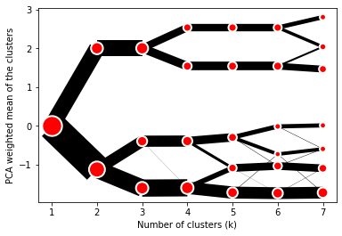 + +## Styling + +`Clustergram.plot()` returns matplotlib axis and can be fully customised as any other +matplotlib plot. + +```python +seaborn.set(style='whitegrid') + +cgram.plot( + ax=ax, + size=0.5, + linewidth=0.5, + cluster_style={"color": "lightblue", "edgecolor": "black"}, + line_style={"color": "red", "linestyle": "-."}, + figsize=(12, 8) +) +``` + +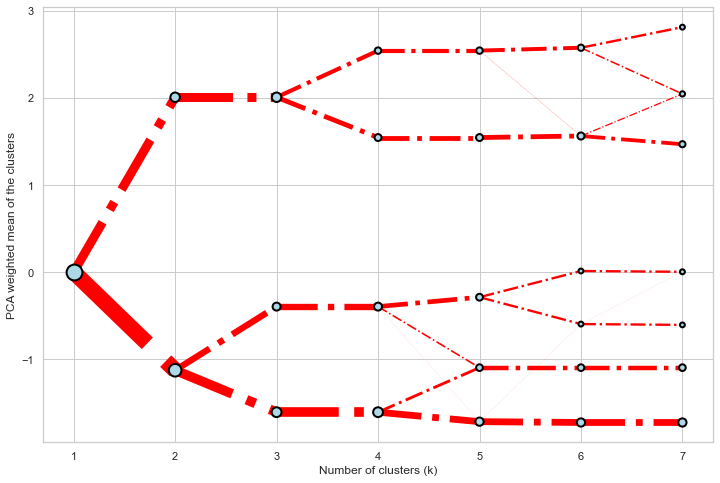 + +## Mean options + +On the `y` axis, a clustergram can use mean values as in the original paper by Matthias +Schonlau or PCA weighted mean values as in the implementation by Tal Galili. + +```python +cgram = Clustergram(range(1, 8)) +cgram.fit(data) +cgram.plot(figsize=(12, 8), pca_weighted=True) +``` + +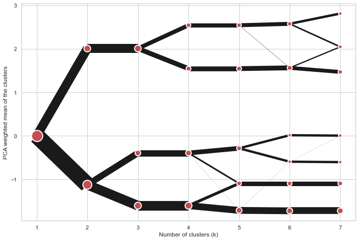 + +```python +cgram = Clustergram(range(1, 8)) +cgram.fit(data) +cgram.plot(figsize=(12, 8), pca_weighted=False) +``` + +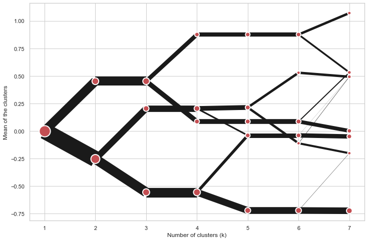 + +## Scikit-learn, SciPy and RAPIDS cuML backends + +Clustergram offers three backends for the computation - `scikit-learn` and `scipy` which +use CPU and RAPIDS.AI `cuML`, which uses GPU. Note that all are optional dependencies +but you will need at least one of them to generate clustergram. + +Using `scikit-learn` (default): + +```python +cgram = Clustergram(range(1, 8), backend='sklearn') +cgram.fit(data) +cgram.plot() +``` + +Using `cuML`: + +```python +cgram = Clustergram(range(1, 8), backend='cuML') +cgram.fit(data) +cgram.plot() +``` + +`data` can be all data types supported by the selected backend (including +`cudf.DataFrame` with `cuML` backend). + +## Supported methods + +Clustergram currently supports K-Means, Mini Batch K-Means, Gaussian Mixture Model and +SciPy's hierarchical clustering methods. Note tha GMM and Mini Batch K-Means are +supported only for `scikit-learn` backend and hierarchical methods are supported only +for `scipy` backend. + +Using K-Means (default): + +```python +cgram = Clustergram(range(1, 8), method='kmeans') +cgram.fit(data) +cgram.plot() +``` + +Using Mini Batch K-Means, which can provide significant speedup over K-Means: + +```python +cgram = Clustergram(range(1, 8), method='minibatchkmeans', batch_size=100) +cgram.fit(data) +cgram.plot() +``` + +Using Gaussian Mixture Model: + +```python +cgram = Clustergram(range(1, 8), method='gmm') +cgram.fit(data) +cgram.plot() +``` + +Using Ward's hierarchical clustering: + +```python +cgram = Clustergram(range(1, 8), method='hierarchical', linkage='ward') +cgram.fit(data) +cgram.plot() +``` + +## Manual input + +Alternatively, you can create clustergram using `from_data` or `from_centers` methods +based on alternative clustering algorithms. + +Using `Clustergram.from_data` which creates cluster centers as mean or median values: + +```python +data = numpy.array([[-1, -1, 0, 10], [1, 1, 10, 2], [0, 0, 20, 4]]) +labels = pandas.DataFrame({1: [0, 0, 0], 2: [0, 0, 1], 3: [0, 2, 1]}) + +cgram = Clustergram.from_data(data, labels) +cgram.plot() +``` + +Using `Clustergram.from_centers` based on explicit cluster centers.: + +```python +labels = pandas.DataFrame({1: [0, 0, 0], 2: [0, 0, 1], 3: [0, 2, 1]}) +centers = { + 1: np.array([[0, 0]]), + 2: np.array([[-1, -1], [1, 1]]), + 3: np.array([[-1, -1], [1, 1], [0, 0]]), + } +cgram = Clustergram.from_centers(centers, labels) +cgram.plot(pca_weighted=False) +``` + +To support PCA weighted plots you also need to pass data: + +```python +cgram = Clustergram.from_centers(centers, labels, data=data) +cgram.plot() +``` + +## Partial plot + +`Clustergram.plot()` can also plot only a part of the diagram, if you want to focus on a +limited range of `k`. + +```python +cgram = Clustergram(range(1, 20)) +cgram.fit(data) +cgram.plot(figsize=(12, 8)) +``` + +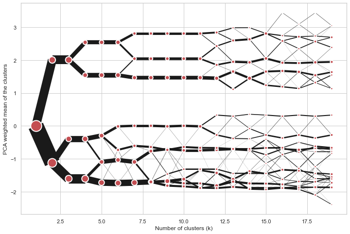 + +```python +cgram.plot(k_range=range(3, 10), figsize=(12, 8)) +``` + +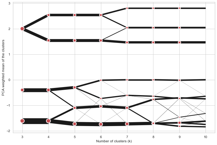 + +## Additional clustering performance evaluation + +Clustergam includes handy wrappers around a selection of clustering performance metrics +offered by `scikit-learn`. Data which were originally computed on GPU are converted to +numpy on the fly. + +### Silhouette score + +Compute the mean Silhouette Coefficient of all samples. See [`scikit-learn` +documentation](https://scikit-learn.org/stable/modules/generated/sklearn.metrics.silhouette_score.html#sklearn.metrics.silhouette_score) +for details. + +```python +>>> cgram.silhouette_score() +2 0.531540 +3 0.447219 +4 0.400154 +5 0.377720 +6 0.372128 +7 0.331575 +Name: silhouette_score, dtype: float64 +``` + +Once computed, resulting Series is available as `cgram.silhouette`. Calling the original +method will recompute the score. + +### Calinski and Harabasz score + +Compute the Calinski and Harabasz score, also known as the Variance Ratio Criterion. See +[`scikit-learn` +documentation](https://scikit-learn.org/stable/modules/generated/sklearn.metrics.calinski_harabasz_score.html#sklearn.metrics.calinski_harabasz_score) +for details. + +```python +>>> cgram.calinski_harabasz_score() +2 482.191469 +3 441.677075 +4 400.392131 +5 411.175066 +6 382.731416 +7 352.447569 +Name: calinski_harabasz_score, dtype: float64 +``` + +Once computed, resulting Series is available as `cgram.calinski_harabasz`. Calling the +original method will recompute the score. + +### Davies-Bouldin score + +Compute the Davies-Bouldin score. See [`scikit-learn` +documentation](https://scikit-learn.org/stable/modules/generated/sklearn.metrics.davies_bouldin_score.html#sklearn.metrics.davies_bouldin_score) +for details. + +```python +>>> cgram.davies_bouldin_score() +2 0.714064 +3 0.943553 +4 0.943320 +5 0.973248 +6 0.950910 +7 1.074937 +Name: davies_bouldin_score, dtype: float64 +``` + +Once computed, resulting Series is available as `cgram.davies_bouldin`. Calling the +original method will recompute the score. + +## Acessing labels + +`Clustergram` stores resulting labels for each of the tested options, which can be +accessed as: + +```python +>>> cgram.labels + 1 2 3 4 5 6 7 +0 0 0 2 2 3 2 1 +1 0 0 2 2 3 2 1 +2 0 0 2 2 3 2 1 +3 0 0 2 2 3 2 1 +4 0 0 2 2 0 0 3 +.. .. .. .. .. .. .. .. +337 0 1 1 3 2 5 0 +338 0 1 1 3 2 5 0 +339 0 1 1 1 1 1 4 +340 0 1 1 3 2 5 5 +341 0 1 1 1 1 1 5 +``` + +## Saving clustergram + +You can save both plot and `clustergram.Clustergram` to a disk. + +### Saving plot + +`Clustergram.plot()` returns matplotlib axis object and as such can be saved as any +other plot: + +```python +import matplotlib.pyplot as plt + +cgram.plot() +plt.savefig('clustergram.svg') +``` + +### Saving object + +If you want to save your computed `clustergram.Clustergram` object to a disk, you can +use `pickle` library: + +```python +import pickle + +with open('clustergram.pickle','wb') as f: + pickle.dump(cgram, f) +``` + +Then loading is equally simple: + +```python +with open('clustergram.pickle','rb') as f: + loaded = pickle.load(f) +``` + +## References + +Schonlau M. The clustergram: a graph for visualizing hierarchical and non-hierarchical +cluster analyses. The Stata Journal, 2002; 2 (4):391-402. + +Schonlau M. Visualizing Hierarchical and Non-Hierarchical Cluster Analyses with +Clustergrams. Computational Statistics: 2004; 19(1):95-111. + +[https://www.r-statistics.com/2010/06/clustergram-visualization-and-diagnostics-for-cluster-analysis-r-code/](https://www.r-statistics.com/2010/06/clustergram-visualization-and-diagnostics-for-cluster-analysis-r-code/) + + +%package -n python3-clustergram +Summary: Clustergram - visualization and diagnostics for cluster analysis +Provides: python-clustergram +BuildRequires: python3-devel +BuildRequires: python3-setuptools +BuildRequires: python3-pip +%description -n python3-clustergram +# Clustergram + + + +## Visualization and diagnostics for cluster analysis + +[](https://doi.org/10.5281/zenodo.4750483) + +Clustergram is a diagram proposed by Matthias Schonlau in his paper *[The clustergram: A +graph for visualizing hierarchical and nonhierarchical cluster +analyses](https://journals.sagepub.com/doi/10.1177/1536867X0200200405)*: + +> In hierarchical cluster analysis, dendrograms are used to visualize how clusters are +> formed. I propose an alternative graph called a “clustergram” to examine how cluster +> members are assigned to clusters as the number of clusters increases. This graph is +> useful in exploratory analysis for nonhierarchical clustering algorithms such as +> k-means and for hierarchical cluster algorithms when the number of observations is +> large enough to make dendrograms impractical. + +The clustergram was later implemented in R by [Tal +Galili](https://www.r-statistics.com/2010/06/clustergram-visualization-and-diagnostics-for-cluster-analysis-r-code/), +who also gives a thorough explanation of the concept. + +This is a Python implementation, originally based on Tal's script, written for +`scikit-learn` and RAPIDS `cuML` implementations of K-Means, Mini Batch K-Means and +Gaussian Mixture Model (scikit-learn only) clustering, plus hierarchical/agglomerative +clustering using `SciPy`. Alternatively, you can create clustergram using `from_*` +constructors based on alternative clustering algorithms. + +[](https://mybinder.org/v2/gh/martinfleis/clustergram/main?urlpath=tree/doc/notebooks/) + +## Getting started + +You can install clustergram from `conda` or `pip`: + +```shell +conda install clustergram -c conda-forge +``` + +```shell +pip install clustergram +``` + +In any case, you still need to install your selected backend (`scikit-learn` and `scipy` +or `cuML`). + +The example of clustergram on Palmer penguins dataset: + +```python +import seaborn +df = seaborn.load_dataset('penguins') +``` + +First we have to select numerical data and scale them. + +```python +from sklearn.preprocessing import scale +data = scale(df.drop(columns=['species', 'island', 'sex']).dropna()) +``` + +And then we can simply pass the data to `clustergram`. + +```python +from clustergram import Clustergram + +cgram = Clustergram(range(1, 8)) +cgram.fit(data) +cgram.plot() +``` + + + +## Styling + +`Clustergram.plot()` returns matplotlib axis and can be fully customised as any other +matplotlib plot. + +```python +seaborn.set(style='whitegrid') + +cgram.plot( + ax=ax, + size=0.5, + linewidth=0.5, + cluster_style={"color": "lightblue", "edgecolor": "black"}, + line_style={"color": "red", "linestyle": "-."}, + figsize=(12, 8) +) +``` + + + +## Mean options + +On the `y` axis, a clustergram can use mean values as in the original paper by Matthias +Schonlau or PCA weighted mean values as in the implementation by Tal Galili. + +```python +cgram = Clustergram(range(1, 8)) +cgram.fit(data) +cgram.plot(figsize=(12, 8), pca_weighted=True) +``` + + + +```python +cgram = Clustergram(range(1, 8)) +cgram.fit(data) +cgram.plot(figsize=(12, 8), pca_weighted=False) +``` + + + +## Scikit-learn, SciPy and RAPIDS cuML backends + +Clustergram offers three backends for the computation - `scikit-learn` and `scipy` which +use CPU and RAPIDS.AI `cuML`, which uses GPU. Note that all are optional dependencies +but you will need at least one of them to generate clustergram. + +Using `scikit-learn` (default): + +```python +cgram = Clustergram(range(1, 8), backend='sklearn') +cgram.fit(data) +cgram.plot() +``` + +Using `cuML`: + +```python +cgram = Clustergram(range(1, 8), backend='cuML') +cgram.fit(data) +cgram.plot() +``` + +`data` can be all data types supported by the selected backend (including +`cudf.DataFrame` with `cuML` backend). + +## Supported methods + +Clustergram currently supports K-Means, Mini Batch K-Means, Gaussian Mixture Model and +SciPy's hierarchical clustering methods. Note tha GMM and Mini Batch K-Means are +supported only for `scikit-learn` backend and hierarchical methods are supported only +for `scipy` backend. + +Using K-Means (default): + +```python +cgram = Clustergram(range(1, 8), method='kmeans') +cgram.fit(data) +cgram.plot() +``` + +Using Mini Batch K-Means, which can provide significant speedup over K-Means: + +```python +cgram = Clustergram(range(1, 8), method='minibatchkmeans', batch_size=100) +cgram.fit(data) +cgram.plot() +``` + +Using Gaussian Mixture Model: + +```python +cgram = Clustergram(range(1, 8), method='gmm') +cgram.fit(data) +cgram.plot() +``` + +Using Ward's hierarchical clustering: + +```python +cgram = Clustergram(range(1, 8), method='hierarchical', linkage='ward') +cgram.fit(data) +cgram.plot() +``` + +## Manual input + +Alternatively, you can create clustergram using `from_data` or `from_centers` methods +based on alternative clustering algorithms. + +Using `Clustergram.from_data` which creates cluster centers as mean or median values: + +```python +data = numpy.array([[-1, -1, 0, 10], [1, 1, 10, 2], [0, 0, 20, 4]]) +labels = pandas.DataFrame({1: [0, 0, 0], 2: [0, 0, 1], 3: [0, 2, 1]}) + +cgram = Clustergram.from_data(data, labels) +cgram.plot() +``` + +Using `Clustergram.from_centers` based on explicit cluster centers.: + +```python +labels = pandas.DataFrame({1: [0, 0, 0], 2: [0, 0, 1], 3: [0, 2, 1]}) +centers = { + 1: np.array([[0, 0]]), + 2: np.array([[-1, -1], [1, 1]]), + 3: np.array([[-1, -1], [1, 1], [0, 0]]), + } +cgram = Clustergram.from_centers(centers, labels) +cgram.plot(pca_weighted=False) +``` + +To support PCA weighted plots you also need to pass data: + +```python +cgram = Clustergram.from_centers(centers, labels, data=data) +cgram.plot() +``` + +## Partial plot + +`Clustergram.plot()` can also plot only a part of the diagram, if you want to focus on a +limited range of `k`. + +```python +cgram = Clustergram(range(1, 20)) +cgram.fit(data) +cgram.plot(figsize=(12, 8)) +``` + + + +```python +cgram.plot(k_range=range(3, 10), figsize=(12, 8)) +``` + + + +## Additional clustering performance evaluation + +Clustergam includes handy wrappers around a selection of clustering performance metrics +offered by `scikit-learn`. Data which were originally computed on GPU are converted to +numpy on the fly. + +### Silhouette score + +Compute the mean Silhouette Coefficient of all samples. See [`scikit-learn` +documentation](https://scikit-learn.org/stable/modules/generated/sklearn.metrics.silhouette_score.html#sklearn.metrics.silhouette_score) +for details. + +```python +>>> cgram.silhouette_score() +2 0.531540 +3 0.447219 +4 0.400154 +5 0.377720 +6 0.372128 +7 0.331575 +Name: silhouette_score, dtype: float64 +``` + +Once computed, resulting Series is available as `cgram.silhouette`. Calling the original +method will recompute the score. + +### Calinski and Harabasz score + +Compute the Calinski and Harabasz score, also known as the Variance Ratio Criterion. See +[`scikit-learn` +documentation](https://scikit-learn.org/stable/modules/generated/sklearn.metrics.calinski_harabasz_score.html#sklearn.metrics.calinski_harabasz_score) +for details. + +```python +>>> cgram.calinski_harabasz_score() +2 482.191469 +3 441.677075 +4 400.392131 +5 411.175066 +6 382.731416 +7 352.447569 +Name: calinski_harabasz_score, dtype: float64 +``` + +Once computed, resulting Series is available as `cgram.calinski_harabasz`. Calling the +original method will recompute the score. + +### Davies-Bouldin score + +Compute the Davies-Bouldin score. See [`scikit-learn` +documentation](https://scikit-learn.org/stable/modules/generated/sklearn.metrics.davies_bouldin_score.html#sklearn.metrics.davies_bouldin_score) +for details. + +```python +>>> cgram.davies_bouldin_score() +2 0.714064 +3 0.943553 +4 0.943320 +5 0.973248 +6 0.950910 +7 1.074937 +Name: davies_bouldin_score, dtype: float64 +``` + +Once computed, resulting Series is available as `cgram.davies_bouldin`. Calling the +original method will recompute the score. + +## Acessing labels + +`Clustergram` stores resulting labels for each of the tested options, which can be +accessed as: + +```python +>>> cgram.labels + 1 2 3 4 5 6 7 +0 0 0 2 2 3 2 1 +1 0 0 2 2 3 2 1 +2 0 0 2 2 3 2 1 +3 0 0 2 2 3 2 1 +4 0 0 2 2 0 0 3 +.. .. .. .. .. .. .. .. +337 0 1 1 3 2 5 0 +338 0 1 1 3 2 5 0 +339 0 1 1 1 1 1 4 +340 0 1 1 3 2 5 5 +341 0 1 1 1 1 1 5 +``` + +## Saving clustergram + +You can save both plot and `clustergram.Clustergram` to a disk. + +### Saving plot + +`Clustergram.plot()` returns matplotlib axis object and as such can be saved as any +other plot: + +```python +import matplotlib.pyplot as plt + +cgram.plot() +plt.savefig('clustergram.svg') +``` + +### Saving object + +If you want to save your computed `clustergram.Clustergram` object to a disk, you can +use `pickle` library: + +```python +import pickle + +with open('clustergram.pickle','wb') as f: + pickle.dump(cgram, f) +``` + +Then loading is equally simple: + +```python +with open('clustergram.pickle','rb') as f: + loaded = pickle.load(f) +``` + +## References + +Schonlau M. The clustergram: a graph for visualizing hierarchical and non-hierarchical +cluster analyses. The Stata Journal, 2002; 2 (4):391-402. + +Schonlau M. Visualizing Hierarchical and Non-Hierarchical Cluster Analyses with +Clustergrams. Computational Statistics: 2004; 19(1):95-111. + +[https://www.r-statistics.com/2010/06/clustergram-visualization-and-diagnostics-for-cluster-analysis-r-code/](https://www.r-statistics.com/2010/06/clustergram-visualization-and-diagnostics-for-cluster-analysis-r-code/) + + +%package help +Summary: Development documents and examples for clustergram +Provides: python3-clustergram-doc +%description help +# Clustergram + + + +## Visualization and diagnostics for cluster analysis + +[](https://doi.org/10.5281/zenodo.4750483) + +Clustergram is a diagram proposed by Matthias Schonlau in his paper *[The clustergram: A +graph for visualizing hierarchical and nonhierarchical cluster +analyses](https://journals.sagepub.com/doi/10.1177/1536867X0200200405)*: + +> In hierarchical cluster analysis, dendrograms are used to visualize how clusters are +> formed. I propose an alternative graph called a “clustergram” to examine how cluster +> members are assigned to clusters as the number of clusters increases. This graph is +> useful in exploratory analysis for nonhierarchical clustering algorithms such as +> k-means and for hierarchical cluster algorithms when the number of observations is +> large enough to make dendrograms impractical. + +The clustergram was later implemented in R by [Tal +Galili](https://www.r-statistics.com/2010/06/clustergram-visualization-and-diagnostics-for-cluster-analysis-r-code/), +who also gives a thorough explanation of the concept. + +This is a Python implementation, originally based on Tal's script, written for +`scikit-learn` and RAPIDS `cuML` implementations of K-Means, Mini Batch K-Means and +Gaussian Mixture Model (scikit-learn only) clustering, plus hierarchical/agglomerative +clustering using `SciPy`. Alternatively, you can create clustergram using `from_*` +constructors based on alternative clustering algorithms. + +[](https://mybinder.org/v2/gh/martinfleis/clustergram/main?urlpath=tree/doc/notebooks/) + +## Getting started + +You can install clustergram from `conda` or `pip`: + +```shell +conda install clustergram -c conda-forge +``` + +```shell +pip install clustergram +``` + +In any case, you still need to install your selected backend (`scikit-learn` and `scipy` +or `cuML`). + +The example of clustergram on Palmer penguins dataset: + +```python +import seaborn +df = seaborn.load_dataset('penguins') +``` + +First we have to select numerical data and scale them. + +```python +from sklearn.preprocessing import scale +data = scale(df.drop(columns=['species', 'island', 'sex']).dropna()) +``` + +And then we can simply pass the data to `clustergram`. + +```python +from clustergram import Clustergram + +cgram = Clustergram(range(1, 8)) +cgram.fit(data) +cgram.plot() +``` + + + +## Styling + +`Clustergram.plot()` returns matplotlib axis and can be fully customised as any other +matplotlib plot. + +```python +seaborn.set(style='whitegrid') + +cgram.plot( + ax=ax, + size=0.5, + linewidth=0.5, + cluster_style={"color": "lightblue", "edgecolor": "black"}, + line_style={"color": "red", "linestyle": "-."}, + figsize=(12, 8) +) +``` + + + +## Mean options + +On the `y` axis, a clustergram can use mean values as in the original paper by Matthias +Schonlau or PCA weighted mean values as in the implementation by Tal Galili. + +```python +cgram = Clustergram(range(1, 8)) +cgram.fit(data) +cgram.plot(figsize=(12, 8), pca_weighted=True) +``` + + + +```python +cgram = Clustergram(range(1, 8)) +cgram.fit(data) +cgram.plot(figsize=(12, 8), pca_weighted=False) +``` + + + +## Scikit-learn, SciPy and RAPIDS cuML backends + +Clustergram offers three backends for the computation - `scikit-learn` and `scipy` which +use CPU and RAPIDS.AI `cuML`, which uses GPU. Note that all are optional dependencies +but you will need at least one of them to generate clustergram. + +Using `scikit-learn` (default): + +```python +cgram = Clustergram(range(1, 8), backend='sklearn') +cgram.fit(data) +cgram.plot() +``` + +Using `cuML`: + +```python +cgram = Clustergram(range(1, 8), backend='cuML') +cgram.fit(data) +cgram.plot() +``` + +`data` can be all data types supported by the selected backend (including +`cudf.DataFrame` with `cuML` backend). + +## Supported methods + +Clustergram currently supports K-Means, Mini Batch K-Means, Gaussian Mixture Model and +SciPy's hierarchical clustering methods. Note tha GMM and Mini Batch K-Means are +supported only for `scikit-learn` backend and hierarchical methods are supported only +for `scipy` backend. + +Using K-Means (default): + +```python +cgram = Clustergram(range(1, 8), method='kmeans') +cgram.fit(data) +cgram.plot() +``` + +Using Mini Batch K-Means, which can provide significant speedup over K-Means: + +```python +cgram = Clustergram(range(1, 8), method='minibatchkmeans', batch_size=100) +cgram.fit(data) +cgram.plot() +``` + +Using Gaussian Mixture Model: + +```python +cgram = Clustergram(range(1, 8), method='gmm') +cgram.fit(data) +cgram.plot() +``` + +Using Ward's hierarchical clustering: + +```python +cgram = Clustergram(range(1, 8), method='hierarchical', linkage='ward') +cgram.fit(data) +cgram.plot() +``` + +## Manual input + +Alternatively, you can create clustergram using `from_data` or `from_centers` methods +based on alternative clustering algorithms. + +Using `Clustergram.from_data` which creates cluster centers as mean or median values: + +```python +data = numpy.array([[-1, -1, 0, 10], [1, 1, 10, 2], [0, 0, 20, 4]]) +labels = pandas.DataFrame({1: [0, 0, 0], 2: [0, 0, 1], 3: [0, 2, 1]}) + +cgram = Clustergram.from_data(data, labels) +cgram.plot() +``` + +Using `Clustergram.from_centers` based on explicit cluster centers.: + +```python +labels = pandas.DataFrame({1: [0, 0, 0], 2: [0, 0, 1], 3: [0, 2, 1]}) +centers = { + 1: np.array([[0, 0]]), + 2: np.array([[-1, -1], [1, 1]]), + 3: np.array([[-1, -1], [1, 1], [0, 0]]), + } +cgram = Clustergram.from_centers(centers, labels) +cgram.plot(pca_weighted=False) +``` + +To support PCA weighted plots you also need to pass data: + +```python +cgram = Clustergram.from_centers(centers, labels, data=data) +cgram.plot() +``` + +## Partial plot + +`Clustergram.plot()` can also plot only a part of the diagram, if you want to focus on a +limited range of `k`. + +```python +cgram = Clustergram(range(1, 20)) +cgram.fit(data) +cgram.plot(figsize=(12, 8)) +``` + + + +```python +cgram.plot(k_range=range(3, 10), figsize=(12, 8)) +``` + + + +## Additional clustering performance evaluation + +Clustergam includes handy wrappers around a selection of clustering performance metrics +offered by `scikit-learn`. Data which were originally computed on GPU are converted to +numpy on the fly. + +### Silhouette score + +Compute the mean Silhouette Coefficient of all samples. See [`scikit-learn` +documentation](https://scikit-learn.org/stable/modules/generated/sklearn.metrics.silhouette_score.html#sklearn.metrics.silhouette_score) +for details. + +```python +>>> cgram.silhouette_score() +2 0.531540 +3 0.447219 +4 0.400154 +5 0.377720 +6 0.372128 +7 0.331575 +Name: silhouette_score, dtype: float64 +``` + +Once computed, resulting Series is available as `cgram.silhouette`. Calling the original +method will recompute the score. + +### Calinski and Harabasz score + +Compute the Calinski and Harabasz score, also known as the Variance Ratio Criterion. See +[`scikit-learn` +documentation](https://scikit-learn.org/stable/modules/generated/sklearn.metrics.calinski_harabasz_score.html#sklearn.metrics.calinski_harabasz_score) +for details. + +```python +>>> cgram.calinski_harabasz_score() +2 482.191469 +3 441.677075 +4 400.392131 +5 411.175066 +6 382.731416 +7 352.447569 +Name: calinski_harabasz_score, dtype: float64 +``` + +Once computed, resulting Series is available as `cgram.calinski_harabasz`. Calling the +original method will recompute the score. + +### Davies-Bouldin score + +Compute the Davies-Bouldin score. See [`scikit-learn` +documentation](https://scikit-learn.org/stable/modules/generated/sklearn.metrics.davies_bouldin_score.html#sklearn.metrics.davies_bouldin_score) +for details. + +```python +>>> cgram.davies_bouldin_score() +2 0.714064 +3 0.943553 +4 0.943320 +5 0.973248 +6 0.950910 +7 1.074937 +Name: davies_bouldin_score, dtype: float64 +``` + +Once computed, resulting Series is available as `cgram.davies_bouldin`. Calling the +original method will recompute the score. + +## Acessing labels + +`Clustergram` stores resulting labels for each of the tested options, which can be +accessed as: + +```python +>>> cgram.labels + 1 2 3 4 5 6 7 +0 0 0 2 2 3 2 1 +1 0 0 2 2 3 2 1 +2 0 0 2 2 3 2 1 +3 0 0 2 2 3 2 1 +4 0 0 2 2 0 0 3 +.. .. .. .. .. .. .. .. +337 0 1 1 3 2 5 0 +338 0 1 1 3 2 5 0 +339 0 1 1 1 1 1 4 +340 0 1 1 3 2 5 5 +341 0 1 1 1 1 1 5 +``` + +## Saving clustergram + +You can save both plot and `clustergram.Clustergram` to a disk. + +### Saving plot + +`Clustergram.plot()` returns matplotlib axis object and as such can be saved as any +other plot: + +```python +import matplotlib.pyplot as plt + +cgram.plot() +plt.savefig('clustergram.svg') +``` + +### Saving object + +If you want to save your computed `clustergram.Clustergram` object to a disk, you can +use `pickle` library: + +```python +import pickle + +with open('clustergram.pickle','wb') as f: + pickle.dump(cgram, f) +``` + +Then loading is equally simple: + +```python +with open('clustergram.pickle','rb') as f: + loaded = pickle.load(f) +``` + +## References + +Schonlau M. The clustergram: a graph for visualizing hierarchical and non-hierarchical +cluster analyses. The Stata Journal, 2002; 2 (4):391-402. + +Schonlau M. Visualizing Hierarchical and Non-Hierarchical Cluster Analyses with +Clustergrams. Computational Statistics: 2004; 19(1):95-111. + +[https://www.r-statistics.com/2010/06/clustergram-visualization-and-diagnostics-for-cluster-analysis-r-code/](https://www.r-statistics.com/2010/06/clustergram-visualization-and-diagnostics-for-cluster-analysis-r-code/) + + +%prep +%autosetup -n clustergram-0.7.0 + +%build +%py3_build + +%install +%py3_install +install -d -m755 %{buildroot}/%{_pkgdocdir} +if [ -d doc ]; then cp -arf doc %{buildroot}/%{_pkgdocdir}; fi +if [ -d docs ]; then cp -arf docs %{buildroot}/%{_pkgdocdir}; fi +if [ -d example ]; then cp -arf example %{buildroot}/%{_pkgdocdir}; fi +if [ -d examples ]; then cp -arf examples %{buildroot}/%{_pkgdocdir}; fi +pushd %{buildroot} +if [ -d usr/lib ]; then + find usr/lib -type f -printf "/%h/%f\n" >> filelist.lst +fi +if [ -d usr/lib64 ]; then + find usr/lib64 -type f -printf "/%h/%f\n" >> filelist.lst +fi +if [ -d usr/bin ]; then + find usr/bin -type f -printf "/%h/%f\n" >> filelist.lst +fi +if [ -d usr/sbin ]; then + find usr/sbin -type f -printf "/%h/%f\n" >> filelist.lst +fi +touch doclist.lst +if [ -d usr/share/man ]; then + find usr/share/man -type f -printf "/%h/%f.gz\n" >> doclist.lst +fi +popd +mv %{buildroot}/filelist.lst . +mv %{buildroot}/doclist.lst . + +%files -n python3-clustergram -f filelist.lst +%dir %{python3_sitelib}/* + +%files help -f doclist.lst +%{_docdir}/* + +%changelog +* Wed May 31 2023 Python_Bot <Python_Bot@openeuler.org> - 0.7.0-1 +- Package Spec generated @@ -0,0 +1 @@ +d612ba4563e6aeffbdac039290428b77 clustergram-0.7.0.tar.gz |