
diff options
| author | CoprDistGit <infra@openeuler.org> | 2023-06-20 06:38:50 +0000 |
|---|---|---|
| committer | CoprDistGit <infra@openeuler.org> | 2023-06-20 06:38:50 +0000 |
| commit | 7d9236b4be8ad4a863ca6b911713cb25d05e3ea0 (patch) | |
| tree | 1aa43b1e3aae30afca16f759c3b39152850ff2c6 | |
| parent | fe5487cf56823fc89e23b40fae53f353e941373f (diff) | |
automatic import of python-sthenoopeneuler20.03
| -rw-r--r-- | .gitignore | 1 | ||||
| -rw-r--r-- | python-stheno.spec | 5453 | ||||
| -rw-r--r-- | sources | 1 |
3 files changed, 5455 insertions, 0 deletions
@@ -0,0 +1 @@ +/stheno-1.4.1.tar.gz diff --git a/python-stheno.spec b/python-stheno.spec new file mode 100644 index 0000000..3bdac69 --- /dev/null +++ b/python-stheno.spec @@ -0,0 +1,5453 @@ +%global _empty_manifest_terminate_build 0 +Name: python-stheno +Version: 1.4.1 +Release: 1 +Summary: Implementation of Gaussian processes in Python +License: MIT +URL: https://github.com/wesselb/stheno +Source0: https://mirrors.aliyun.com/pypi/web/packages/ef/57/40ad77b4b8b86e8438bba233f843d6da50d178b7f2ad8c30151314a1ac4c/stheno-1.4.1.tar.gz +BuildArch: noarch + +Requires: python3-numpy +Requires: python3-fdm +Requires: python3-algebra +Requires: python3-plum-dispatch +Requires: python3-backends +Requires: python3-backends-matrix +Requires: python3-mlkernels +Requires: python3-wbml + +%description +# [Stheno](https://github.com/wesselb/stheno) + +[](https://github.com/wesselb/stheno/actions?query=workflow%3ACI) +[](https://coveralls.io/github/wesselb/stheno?branch=master) +[](https://wesselb.github.io/stheno) +[](https://github.com/psf/black) + +Stheno is an implementation of Gaussian process modelling in Python. See +also [Stheno.jl](https://github.com/willtebbutt/Stheno.jl). + +[Check out our post about linear models with Stheno and JAX.](https://wesselb.github.io/2021/01/19/linear-models-with-stheno-and-jax.html) + +Contents: + +* [Nonlinear Regression in 20 Seconds](#nonlinear-regression-in-20-seconds) +* [Installation](#installation) +* [Manual](#manual) + - [AutoGrad, TensorFlow, PyTorch, or JAX? Your Choice!](#autograd-tensorflow-pytorch-or-jax-your-choice) + - [Model Design](#model-design) + - [Finite-Dimensional Distributions](#finite-dimensional-distributions) + - [Prior and Posterior Measures](#prior-and-posterior-measures) + - [Inducing Points](#inducing-points) + - [Kernels and Means](#kernels-and-means) + - [Batched Computation](#batched-computation) + - [Important Remarks](#important-remarks) +* [Examples](#examples) + - [Simple Regression](#simple-regression) + - [Hyperparameter Optimisation with Varz](#hyperparameter-optimisation-with-varz) + - [Hyperparameter Optimisation with PyTorch](#hyperparameter-optimisation-with-pytorch) + - [Decomposition of Prediction](#decomposition-of-prediction) + - [Learn a Function, Incorporating Prior Knowledge About Its Form](#learn-a-function-incorporating-prior-knowledge-about-its-form) + - [Multi-Output Regression](#multi-output-regression) + - [Approximate Integration](#approximate-integration) + - [Bayesian Linear Regression](#bayesian-linear-regression) + - [GPAR](#gpar) + - [A GP-RNN Model](#a-gp-rnn-model) + - [Approximate Multiplication Between GPs](#approximate-multiplication-between-gps) + - [Sparse Regression](#sparse-regression) + - [Smoothing with Nonparametric Basis Functions](#smoothing-with-nonparametric-basis-functions) + +## Nonlinear Regression in 20 Seconds + +```python +>>> import numpy as np + +>>> from stheno import GP, EQ + +>>> x = np.linspace(0, 2, 10) # Some points to predict at + +>>> y = x ** 2 # Some observations + +>>> f = GP(EQ()) # Construct Gaussian process. + +>>> f_post = f | (f(x), y) # Compute the posterior. + +>>> pred = f_post(np.array([1, 2, 3])) # Predict! + +>>> pred.mean +<dense matrix: shape=3x1, dtype=float64 + mat=[[1. ] + [4. ] + [8.483]]> + +>>> pred.var +<dense matrix: shape=3x3, dtype=float64 + mat=[[ 8.032e-13 7.772e-16 -4.577e-09] + [ 7.772e-16 9.999e-13 2.773e-10] + [-4.577e-09 2.773e-10 3.313e-03]]> +``` + +[These custom matrix types are there to accelerate the underlying linear algebra.](#important-remarks) +To get vanilla NumPy/AutoGrad/TensorFlow/PyTorch/JAX arrays, use `B.dense`: + +```python +>>> from lab import B + +>>> B.dense(pred.mean) +array([[1.00000068], + [3.99999999], + [8.4825932 ]]) + +>>> B.dense(pred.var) +array([[ 8.03246358e-13, 7.77156117e-16, -4.57690943e-09], + [ 7.77156117e-16, 9.99866856e-13, 2.77333267e-10], + [-4.57690943e-09, 2.77333267e-10, 3.31283378e-03]]) +``` + +Moar?! Then read on! + +## Installation + +See [the instructions here](https://gist.github.com/wesselb/4b44bf87f3789425f96e26c4308d0adc). +Then simply + +``` +pip install stheno +``` + +## Manual + +Note: [here](https://wesselb.github.io/stheno) is a nicely rendered and more +readable version of the docs. + +### AutoGrad, TensorFlow, PyTorch, or JAX? Your Choice! + +```python +from stheno.autograd import GP, EQ +``` + +```python +from stheno.tensorflow import GP, EQ +``` + +```python +from stheno.torch import GP, EQ +``` + +```python +from stheno.jax import GP, EQ +``` + +### Model Design + +The basic building block is a `f = GP(mean=0, kernel, measure=prior)`, which takes +in [a _mean_, a _kernel_](#kernels-and-means), and a _measure_. +The mean and kernel of a GP can be extracted with `f.mean` and `f.kernel`. +The measure should be thought of as a big joint distribution that assigns a mean and +a kernel to every variable `f`. +A measure can be created with `prior = Measure()`. +A GP `f` can have different means and kernels under different measures. +For example, under some _prior_ measure, `f` can have an `EQ()` kernel; but, under some +_posterior_ measure, `f` has a kernel that is determined by the posterior distribution +of a GP. +[We will see later how posterior measures can be constructed.](#prior-and-posterior-measures) +The measure with which a `f = GP(kernel, measure=prior)` is constructed can be +extracted with `f.measure == prior`. +If the keyword argument `measure` is not set, then automatically a new measure is +created, which afterwards can be extracted with `f.measure`. + +Definition, where `prior = Measure()`: + +```python +f = GP(kernel) + +f = GP(mean, kernel) + +f = GP(kernel, measure=prior) + +f = GP(mean, kernel, measure=prior) +``` + +GPs that are associated to the same measure can be combined into new GPs, which is +the primary mechanism used to build cool models. + +Here's an example model: + +```python +>>> prior = Measure() + +>>> f1 = GP(lambda x: x ** 2, EQ(), measure=prior) + +>>> f1 +GP(<lambda>, EQ()) + +>>> f2 = GP(Linear(), measure=prior) + +>>> f2 +GP(0, Linear()) + +>>> f_sum = f1 + f2 + +>>> f_sum +GP(<lambda>, EQ() + Linear()) + +>>> f_sum + GP(EQ()) # Not valid: `GP(EQ())` belongs to a new measure! +AssertionError: Processes GP(<lambda>, EQ() + Linear()) and GP(0, EQ()) are associated to different measures. +``` + +To avoid setting the keyword `measure` for every `GP` that you create, you can enter +a measure as a context: + +```python +>>> with Measure() as prior: + f1 = GP(lambda x: x ** 2, EQ()) + f2 = GP(Linear()) + f_sum = f1 + f2 + +>>> prior == f1.measure == f2.measure == f_sum.measure +True +``` + + + +#### Compositional Design + +* Add and subtract GPs and other objects. + + Example: + + ```python + >>> GP(EQ(), measure=prior) + GP(Exp(), measure=prior) + GP(0, EQ() + Exp()) + + >>> GP(EQ(), measure=prior) + GP(EQ(), measure=prior) + GP(0, 2 * EQ()) + + >>> GP(EQ()) + 1 + GP(1, EQ()) + + >>> GP(EQ()) + 0 + GP(0, EQ()) + + >>> GP(EQ()) + (lambda x: x ** 2) + GP(<lambda>, EQ()) + + >>> GP(2, EQ(), measure=prior) - GP(1, EQ(), measure=prior) + GP(1, 2 * EQ()) + ``` + +* Multiply GPs and other objects. + + *Warning:* + The product of two GPs it *not* a Gaussian process. + Stheno approximates the resulting process by moment matching. + + Example: + + ```python + >>> GP(1, EQ(), measure=prior) * GP(1, Exp(), measure=prior) + GP(<lambda> + <lambda> + -1 * 1, <lambda> * Exp() + <lambda> * EQ() + EQ() * Exp()) + + >>> 2 * GP(EQ()) + GP(2, 2 * EQ()) + + >>> 0 * GP(EQ()) + GP(0, 0) + + >>> (lambda x: x) * GP(EQ()) + GP(0, <lambda> * EQ()) + ``` + +* Shift GPs. + + Example: + + ```python + >>> GP(EQ()).shift(1) + GP(0, EQ() shift 1) + ``` + +* Stretch GPs. + + Example: + + ```python + >>> GP(EQ()).stretch(2) + GP(0, EQ() > 2) + ``` + +* Select particular input dimensions. + + Example: + + ```python + >>> GP(EQ()).select(1, 3) + GP(0, EQ() : [1, 3]) + ``` + +* Transform the input. + + Example: + + ```python + >>> GP(EQ()).transform(f) + GP(0, EQ() transform f) + ``` + +* Numerically take the derivative of a GP. + The argument specifies which dimension to take the derivative with respect + to. + + Example: + + ```python + >>> GP(EQ()).diff(1) + GP(0, d(1) EQ()) + ``` + +* Construct a finite difference estimate of the derivative of a GP. + See `Measure.diff_approx` for a description of the arguments. + + Example: + + ```python + >>> GP(EQ()).diff_approx(deriv=1, order=2) + GP(50000000.0 * (0.5 * EQ() + 0.5 * ((-0.5 * (EQ() shift (0.0001414213562373095, 0))) shift (0, -0.0001414213562373095)) + 0.5 * ((-0.5 * (EQ() shift (0, 0.0001414213562373095))) shift (-0.0001414213562373095, 0))), 0) + ``` + +* Construct the Cartesian product of a collection of GPs. + + Example: + + ```python + >>> prior = Measure() + + >>> f1, f2 = GP(EQ(), measure=prior), GP(EQ(), measure=prior) + + >>> cross(f1, f2) + GP(MultiOutputMean(0, 0), MultiOutputKernel(EQ(), EQ())) + ``` + +#### Displaying GPs + +GPs have a `display` method that accepts a formatter. + +Example: + +```python +>>> print(GP(2.12345 * EQ()).display(lambda x: f"{x:.2f}")) +GP(2.12 * EQ(), 0) +``` + +#### Properties of GPs + +[Properties of kernels](https://github.com/wesselb/mlkernels#properties-of-kernels-and-means) +can be queried on GPs directly. + +Example: + +```python +>>> GP(EQ()).stationary +True +``` + +#### Naming GPs + +It is possible to give a name to a GP. +Names must be strings. +A measure then behaves like a two-way dictionary between GPs and their names. + +Example: + +```python +>>> prior = Measure() + +>>> p = GP(EQ(), name="name", measure=prior) + +>>> p.name +'name' + +>>> p.name = "alternative_name" + +>>> prior["alternative_name"] +GP(0, EQ()) + +>>> prior[p] +'alternative_name' +``` + +### Finite-Dimensional Distributions + +Simply call a GP to construct a finite-dimensional distribution at some inputs. +You can give a second argument, which specifies the variance of additional additive +noise. +After constructing a finite-dimensional distribution, you can compute the mean, +the variance, sample, or compute a logpdf. + +Definition, where `f` is a `GP`: + +```python +f(x) # No additional noise + +f(x, noise) # Additional noise with variance `noise` +``` + +Things you can do with a finite-dimensional distribution: + +* + Use `f(x).mean` to compute the mean. + +* + Use `f(x).var` to compute the variance. + +* + Use `f(x).mean_var` to compute simultaneously compute the mean and variance. + This can be substantially more efficient than calling first `f(x).mean` and then + `f(x).var`. + +* + Use `Normal.sample` to sample. + + Definition: + + ```python + f(x).sample() # Produce one sample. + + f(x).sample(n) # Produce `n` samples. + + f(x).sample(noise=noise) # Produce one samples with additional noise variance `noise`. + + f(x).sample(n, noise=noise) # Produce `n` samples with additional noise variance `noise`. + ``` + +* + Use `f(x).logpdf(y)` to compute the logpdf of some data `y`. + +* + Use `means, variances = f(x).marginals()` to efficiently compute the marginal means + and marginal variances. + + Example: + + ```python + >>> f(x).marginals() + (array([0., 0., 0.]), np.array([1., 1., 1.])) + ``` + +* + Use `means, lowers, uppers = f(x).marginal_credible_bounds()` to efficiently compute + the means and the marginal lower and upper 95% central credible region bounds. + + Example: + + ```python + >>> f(x).marginal_credible_bounds() + (array([0., 0., 0.]), array([-1.96, -1.96, -1.96]), array([1.96, 1.96, 1.96])) + ``` + +* + Use `Measure.logpdf` to compute the joint logpdf of multiple observations. + + Definition, where `prior = Measure()`: + + ```python + prior.logpdf(f(x), y) + + prior.logpdf((f1(x1), y1), (f2(x2), y2), ...) + ``` + +* + Use `Measure.sample` to jointly sample multiple observations. + + Definition, where `prior = Measure()`: + + ```python + sample = prior.sample(f(x)) + + sample1, sample2, ... = prior.sample(f1(x1), f2(x2), ...) + ``` + +Example: + +```python +>>> prior = Measure() + +>>> f = GP(EQ(), measure=prior) + +>>> x = np.array([0., 1., 2.]) + +>>> f(x) # FDD without noise. +<FDD: + process=GP(0, EQ()), + input=array([0., 1., 2.]), + noise=<zero matrix: shape=3x3, dtype=float64> + +>>> f(x, 0.1) # FDD with noise. +<FDD: + process=GP(0, EQ()), + input=array([0., 1., 2.]), + noise=<diagonal matrix: shape=3x3, dtype=float64 + diag=[0.1 0.1 0.1]>> + +>>> f(x).mean +array([[0.], + [0.], + [0.]]) + +>>> f(x).var +<dense matrix: shape=3x3, dtype=float64 + mat=[[1. 0.607 0.135] + [0.607 1. 0.607] + [0.135 0.607 1. ]]> + +>>> y1 = f(x).sample() + +>>> y1 +array([[-0.45172746], + [ 0.46581948], + [ 0.78929767]]) + +>>> f(x).logpdf(y1) +-2.811609567720761 + +>>> y2 = f(x).sample(2) +array([[-0.43771276, -2.36741858], + [ 0.86080043, -1.22503079], + [ 2.15779126, -0.75319405]] + +>>> f(x).logpdf(y2) + array([-4.82949038, -5.40084225]) +``` + +### Prior and Posterior Measures + +Conditioning a _prior_ measure on observations gives a _posterior_ measure. +To condition a measure on observations, use `Measure.__or__`. + +Definition, where `prior = Measure()` and `f*` are `GP`s: + +```python +post = prior | (f(x, [noise]), y) + +post = prior | ((f1(x1, [noise1]), y1), (f2(x2, [noise2]), y2), ...) +``` + +You can then obtain a posterior process with `post(f)` and a finite-dimensional +distribution under the posterior with `post(f(x))`. +Alternatively, the posterior of a process `f` can be obtained by conditioning `f` +directly. + +Definition, where and `f*` are `GP`s: + +```python +f_post = f | (f(x, [noise]), y) + +f_post = f | ((f1(x1, [noise1]), y1), (f2(x2, [noise2]), y2), ...) +``` + +Let's consider an example. +First, build a model and sample some values. + +```python +>>> prior = Measure() + +>>> f = GP(EQ(), measure=prior) + +>>> x = np.array([0., 1., 2.]) + +>>> y = f(x).sample() +``` + +Then compute the posterior measure. + +```python +>>> post = prior | (f(x), y) + +>>> post(f) +GP(PosteriorMean(), PosteriorKernel()) + +>>> post(f).mean(x) +<dense matrix: shape=3x1, dtype=float64 + mat=[[ 0.412] + [-0.811] + [-0.933]]> + +>>> post(f).kernel(x) +<dense matrix: shape=3x3, dtype=float64 + mat=[[1.e-12 0.e+00 0.e+00] + [0.e+00 1.e-12 0.e+00] + [0.e+00 0.e+00 1.e-12]]> + +>>> post(f(x)) +<FDD: + process=GP(PosteriorMean(), PosteriorKernel()), + input=array([0., 1., 2.]), + noise=<zero matrix: shape=3x3, dtype=float64>> + +>>> post(f(x)).mean +<dense matrix: shape=3x1, dtype=float64 + mat=[[ 0.412] + [-0.811] + [-0.933]]> + +>>> post(f(x)).var +<dense matrix: shape=3x3, dtype=float64 + mat=[[1.e-12 0.e+00 0.e+00] + [0.e+00 1.e-12 0.e+00] + [0.e+00 0.e+00 1.e-12]]> +``` + +We can also obtain the posterior by conditioning `f` directly: + +```python +>>> f_post = f | (f(x), y) + +>>> f_post +GP(PosteriorMean(), PosteriorKernel()) + +>>> f_post.mean(x) +<dense matrix: shape=3x1, dtype=float64 + mat=[[ 0.412] + [-0.811] + [-0.933]]> + +>>> f_post.kernel(x) +<dense matrix: shape=3x3, dtype=float64 + mat=[[1.e-12 0.e+00 0.e+00] + [0.e+00 1.e-12 0.e+00] + [0.e+00 0.e+00 1.e-12]]> + +>>> f_post(x) +<FDD: + process=GP(PosteriorMean(), PosteriorKernel()), + input=array([0., 1., 2.]), + noise=<zero matrix: shape=3x3, dtype=float64>> + +>>> f_post(x).mean +<dense matrix: shape=3x1, dtype=float64 + mat=[[ 0.412] + [-0.811] + [-0.933]]> + +>>> f_post(x).var +<dense matrix: shape=3x3, dtype=float64 + mat=[[1.e-12 0.e+00 0.e+00] + [0.e+00 1.e-12 0.e+00] + [0.e+00 0.e+00 1.e-12]]> +``` + +We can further extend our model by building on the posterior. + +```python +>>> g = GP(Linear(), measure=post) + +>>> f_sum = post(f) + g + +>>> f_sum +GP(PosteriorMean(), PosteriorKernel() + Linear()) +``` + +However, what we cannot do is mixing the prior and posterior. + +```python +>>> f + g +AssertionError: Processes GP(0, EQ()) and GP(0, Linear()) are associated to different measures. +``` + +### Inducing Points + +Stheno supports pseudo-point approximations of posterior distributions with +various approximation methods: + +1. The Variational Free Energy (VFE; + [Titsias, 2009](http://proceedings.mlr.press/v5/titsias09a/titsias09a.pdf)) + approximation. + To use the VFE approximation, use `PseudoObs`. + +2. The Fully Independent Training Conditional (FITC; + [Snelson & Ghahramani, 2006](http://www.gatsby.ucl.ac.uk/~snelson/SPGP_up.pdf)) + approximation. + To use the FITC approximation, use `PseudoObsFITC`. + +3. The Deterministic Training Conditional (DTC; + [Csato & Opper, 2002](https://direct.mit.edu/neco/article/14/3/641/6594/Sparse-On-Line-Gaussian-Processes); + [Seeger et al., 2003](http://proceedings.mlr.press/r4/seeger03a/seeger03a.pdf)) + approximation. + To use the DTC approximation, use `PseudoObsDTC`. + +The VFE approximation (`PseudoObs`) is the approximation recommended to use. +The following definitions and examples will use the VFE approximation with `PseudoObs`, +but every instance of `PseudoObs` can be swapped out for `PseudoObsFITC` or +`PseudoObsDTC`. + +Definition: + +```python +obs = PseudoObs( + u(z), # FDD of inducing points + (f(x, [noise]), y) # Observed data +) + +obs = PseudoObs(u(z), f(x, [noise]), y) + +obs = PseudoObs(u(z), (f1(x1, [noise1]), y1), (f2(x2, [noise2]), y2), ...) + +obs = PseudoObs((u1(z1), u2(z2), ...), f(x, [noise]), y) + +obs = PseudoObs((u1(z1), u2(z2), ...), (f1(x1, [noise1]), y1), (f2(x2, [noise2]), y2), ...) +``` + +The approximate posterior measure can be constructed with `prior | obs` +where `prior = Measure()` is the measure of your model. +To quantify the quality of the approximation, you can compute the ELBO with +`obs.elbo(prior)`. + +Let's consider an example. +First, build a model and sample some noisy observations. + +```python +>>> prior = Measure() + +>>> f = GP(EQ(), measure=prior) + +>>> x_obs = np.linspace(0, 10, 2000) + +>>> y_obs = f(x_obs, 1).sample() +``` + +Ouch, computing the logpdf is quite slow: + +```python +>>> %timeit f(x_obs, 1).logpdf(y_obs) +219 ms ± 35.7 ms per loop (mean ± std. dev. of 7 runs, 10 loops each) +``` + +Let's try to use inducing points to speed this up. + +```python +>>> x_ind = np.linspace(0, 10, 100) + +>>> u = f(x_ind) # FDD of inducing points. + +>>> %timeit PseudoObs(u, f(x_obs, 1), y_obs).elbo(prior) +9.8 ms ± 181 µs per loop (mean ± std. dev. of 7 runs, 100 loops each) +``` + +Much better. +And the approximation is good: + +```python +>>> PseudoObs(u, f(x_obs, 1), y_obs).elbo(prior) - f(x_obs, 1).logpdf(y_obs) +-3.537934389896691e-10 +``` + +We finally construct the approximate posterior measure: + +```python +>>> post_approx = prior | PseudoObs(u, f(x_obs, 1), y_obs) + +>>> post_approx(f(x_obs)).mean +<dense matrix: shape=2000x1, dtype=float64 + mat=[[0.469] + [0.468] + [0.467] + ... + [1.09 ] + [1.09 ] + [1.091]]> +``` + + +### Kernels and Means + +See [MLKernels](https://github.com/wesselb/mlkernels). + + +### Batched Computation + +Stheno supports batched computation. +See [MLKernels](https://github.com/wesselb/mlkernels/#usage) for a description of how +means and kernels work with batched computation. + +Example: + +```python +>>> f = GP(EQ()) + +>>> x = np.random.randn(16, 100, 1) + +>>> y = f(x, 1).sample() + +>>> logpdf = f(x, 1).logpdf(y) + +>>> y.shape +(16, 100, 1) + +>>> f(x, 1).logpdf(y).shape +(16,) +``` + + +### Important Remarks + +Stheno uses [LAB](https://github.com/wesselb/lab) to provide an implementation that is +backend agnostic. +Moreover, Stheno uses [an extension of LAB](https://github.com/wesselb/matrix) to +accelerate linear algebra with structured linear algebra primitives. +You will encounter these primitives: + +```python +>>> k = 2 * Delta() + +>>> x = np.linspace(0, 5, 10) + +>>> k(x) +<diagonal matrix: shape=10x10, dtype=float64 + diag=[2. 2. 2. 2. 2. 2. 2. 2. 2. 2.]> +``` + +If you're using [LAB](https://github.com/wesselb/lab) to further process these matrices, +then there is absolutely no need to worry: +these structured matrix types know how to add, multiply, and do other linear algebra +operations. + +```python +>>> import lab as B + +>>> B.matmul(k(x), k(x)) +<diagonal matrix: shape=10x10, dtype=float64 + diag=[4. 4. 4. 4. 4. 4. 4. 4. 4. 4.]> +``` + +If you're not using [LAB](https://github.com/wesselb/lab), you can convert these +structured primitives to regular NumPy/TensorFlow/PyTorch/JAX arrays by calling +`B.dense` (`B` is from [LAB](https://github.com/wesselb/lab)): + +```python +>>> import lab as B + +>>> B.dense(k(x)) +array([[2., 0., 0., 0., 0., 0., 0., 0., 0., 0.], + [0., 2., 0., 0., 0., 0., 0., 0., 0., 0.], + [0., 0., 2., 0., 0., 0., 0., 0., 0., 0.], + [0., 0., 0., 2., 0., 0., 0., 0., 0., 0.], + [0., 0., 0., 0., 2., 0., 0., 0., 0., 0.], + [0., 0., 0., 0., 0., 2., 0., 0., 0., 0.], + [0., 0., 0., 0., 0., 0., 2., 0., 0., 0.], + [0., 0., 0., 0., 0., 0., 0., 2., 0., 0.], + [0., 0., 0., 0., 0., 0., 0., 0., 2., 0.], + [0., 0., 0., 0., 0., 0., 0., 0., 0., 2.]]) +``` + +Furthermore, before computing a Cholesky decomposition, Stheno always adds a minuscule +diagonal to prevent the Cholesky decomposition from failing due to positive +indefiniteness caused by numerical noise. +You can change the magnitude of this diagonal by changing `B.epsilon`: + +```python +>>> import lab as B + +>>> B.epsilon = 1e-12 # Default regularisation + +>>> B.epsilon = 1e-8 # Strong regularisation +``` + + +## Examples + +The examples make use of [Varz](https://github.com/wesselb/varz) and some +utility from [WBML](https://github.com/wesselb/wbml). + + +### Simple Regression + +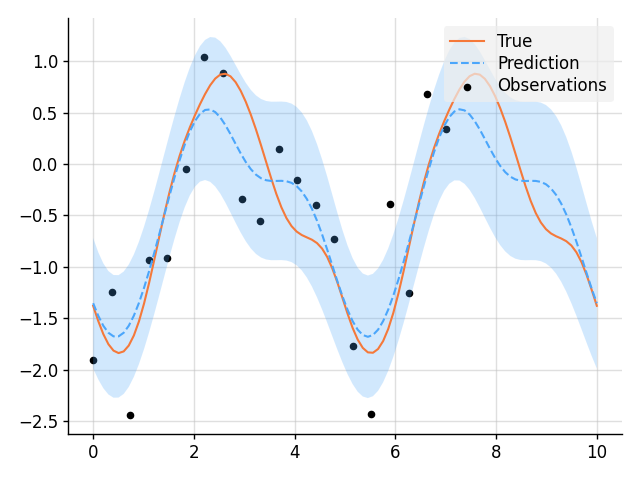 + +```python +import matplotlib.pyplot as plt +from wbml.plot import tweak + +from stheno import B, GP, EQ + +# Define points to predict at. +x = B.linspace(0, 10, 100) +x_obs = B.linspace(0, 7, 20) + +# Construct a prior. +f = GP(EQ().periodic(5.0)) + +# Sample a true, underlying function and noisy observations. +f_true, y_obs = f.measure.sample(f(x), f(x_obs, 0.5)) + +# Now condition on the observations to make predictions. +f_post = f | (f(x_obs, 0.5), y_obs) +mean, lower, upper = f_post(x).marginal_credible_bounds() + +# Plot result. +plt.plot(x, f_true, label="True", style="test") +plt.scatter(x_obs, y_obs, label="Observations", style="train", s=20) +plt.plot(x, mean, label="Prediction", style="pred") +plt.fill_between(x, lower, upper, style="pred") +tweak() +plt.savefig("readme_example1_simple_regression.png") +plt.show() +``` + +### Hyperparameter Optimisation with Varz + +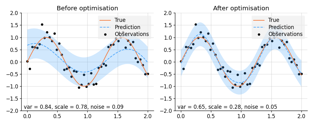 + +```python +import lab as B +import matplotlib.pyplot as plt +import torch +from varz import Vars, minimise_l_bfgs_b, parametrised, Positive +from wbml.plot import tweak + +from stheno.torch import EQ, GP + +# Increase regularisation because PyTorch defaults to 32-bit floats. +B.epsilon = 1e-6 + +# Define points to predict at. +x = torch.linspace(0, 2, 100) +x_obs = torch.linspace(0, 2, 50) + +# Sample a true, underlying function and observations with observation noise `0.05`. +f_true = torch.sin(5 * x) +y_obs = torch.sin(5 * x_obs) + 0.05**0.5 * torch.randn(50) + + +def model(vs): + """Construct a model with learnable parameters.""" + p = vs.struct # Varz handles positivity (and other) constraints. + kernel = p.variance.positive() * EQ().stretch(p.scale.positive()) + return GP(kernel), p.noise.positive() + + +@parametrised +def model_alternative(vs, scale: Positive, variance: Positive, noise: Positive): + """Equivalent to :func:`model`, but with `@parametrised`.""" + kernel = variance * EQ().stretch(scale) + return GP(kernel), noise + + +vs = Vars(torch.float32) +f, noise = model(vs) + +# Condition on observations and make predictions before optimisation. +f_post = f | (f(x_obs, noise), y_obs) +prior_before = f, noise +pred_before = f_post(x, noise).marginal_credible_bounds() + + +def objective(vs): + f, noise = model(vs) + evidence = f(x_obs, noise).logpdf(y_obs) + return -evidence + + +# Learn hyperparameters. +minimise_l_bfgs_b(objective, vs) + +f, noise = model(vs) + +# Condition on observations and make predictions after optimisation. +f_post = f | (f(x_obs, noise), y_obs) +prior_after = f, noise +pred_after = f_post(x, noise).marginal_credible_bounds() + + +def plot_prediction(prior, pred): + f, noise = prior + mean, lower, upper = pred + plt.scatter(x_obs, y_obs, label="Observations", style="train", s=20) + plt.plot(x, f_true, label="True", style="test") + plt.plot(x, mean, label="Prediction", style="pred") + plt.fill_between(x, lower, upper, style="pred") + plt.ylim(-2, 2) + plt.text( + 0.02, + 0.02, + f"var = {f.kernel.factor(0):.2f}, " + f"scale = {f.kernel.factor(1).stretches[0]:.2f}, " + f"noise = {noise:.2f}", + transform=plt.gca().transAxes, + ) + tweak() + + +# Plot result. +plt.figure(figsize=(10, 4)) +plt.subplot(1, 2, 1) +plt.title("Before optimisation") +plot_prediction(prior_before, pred_before) +plt.subplot(1, 2, 2) +plt.title("After optimisation") +plot_prediction(prior_after, pred_after) +plt.savefig("readme_example12_optimisation_varz.png") +plt.show() +``` + +### Hyperparameter Optimisation with PyTorch + +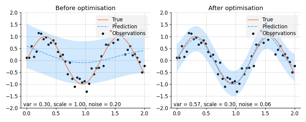 + +```python +import lab as B +import matplotlib.pyplot as plt +import torch +from wbml.plot import tweak + +from stheno.torch import EQ, GP + +# Increase regularisation because PyTorch defaults to 32-bit floats. +B.epsilon = 1e-6 + +# Define points to predict at. +x = torch.linspace(0, 2, 100) +x_obs = torch.linspace(0, 2, 50) + +# Sample a true, underlying function and observations with observation noise `0.05`. +f_true = torch.sin(5 * x) +y_obs = torch.sin(5 * x_obs) + 0.05**0.5 * torch.randn(50) + + +class Model(torch.nn.Module): + """A GP model with learnable parameters.""" + + def __init__(self, init_var=0.3, init_scale=1, init_noise=0.2): + super().__init__() + # Ensure that the parameters are positive and make them learnable. + self.log_var = torch.nn.Parameter(torch.log(torch.tensor(init_var))) + self.log_scale = torch.nn.Parameter(torch.log(torch.tensor(init_scale))) + self.log_noise = torch.nn.Parameter(torch.log(torch.tensor(init_noise))) + + def construct(self): + self.var = torch.exp(self.log_var) + self.scale = torch.exp(self.log_scale) + self.noise = torch.exp(self.log_noise) + kernel = self.var * EQ().stretch(self.scale) + return GP(kernel), self.noise + + +model = Model() +f, noise = model.construct() + +# Condition on observations and make predictions before optimisation. +f_post = f | (f(x_obs, noise), y_obs) +prior_before = f, noise +pred_before = f_post(x, noise).marginal_credible_bounds() + +# Perform optimisation. +opt = torch.optim.Adam(model.parameters(), lr=5e-2) +for _ in range(1000): + opt.zero_grad() + f, noise = model.construct() + loss = -f(x_obs, noise).logpdf(y_obs) + loss.backward() + opt.step() + +f, noise = model.construct() + +# Condition on observations and make predictions after optimisation. +f_post = f | (f(x_obs, noise), y_obs) +prior_after = f, noise +pred_after = f_post(x, noise).marginal_credible_bounds() + + +def plot_prediction(prior, pred): + f, noise = prior + mean, lower, upper = pred + plt.scatter(x_obs, y_obs, label="Observations", style="train", s=20) + plt.plot(x, f_true, label="True", style="test") + plt.plot(x, mean, label="Prediction", style="pred") + plt.fill_between(x, lower, upper, style="pred") + plt.ylim(-2, 2) + plt.text( + 0.02, + 0.02, + f"var = {f.kernel.factor(0):.2f}, " + f"scale = {f.kernel.factor(1).stretches[0]:.2f}, " + f"noise = {noise:.2f}", + transform=plt.gca().transAxes, + ) + tweak() + + +# Plot result. +plt.figure(figsize=(10, 4)) +plt.subplot(1, 2, 1) +plt.title("Before optimisation") +plot_prediction(prior_before, pred_before) +plt.subplot(1, 2, 2) +plt.title("After optimisation") +plot_prediction(prior_after, pred_after) +plt.savefig("readme_example13_optimisation_torch.png") +plt.show() +``` + +### Decomposition of Prediction + +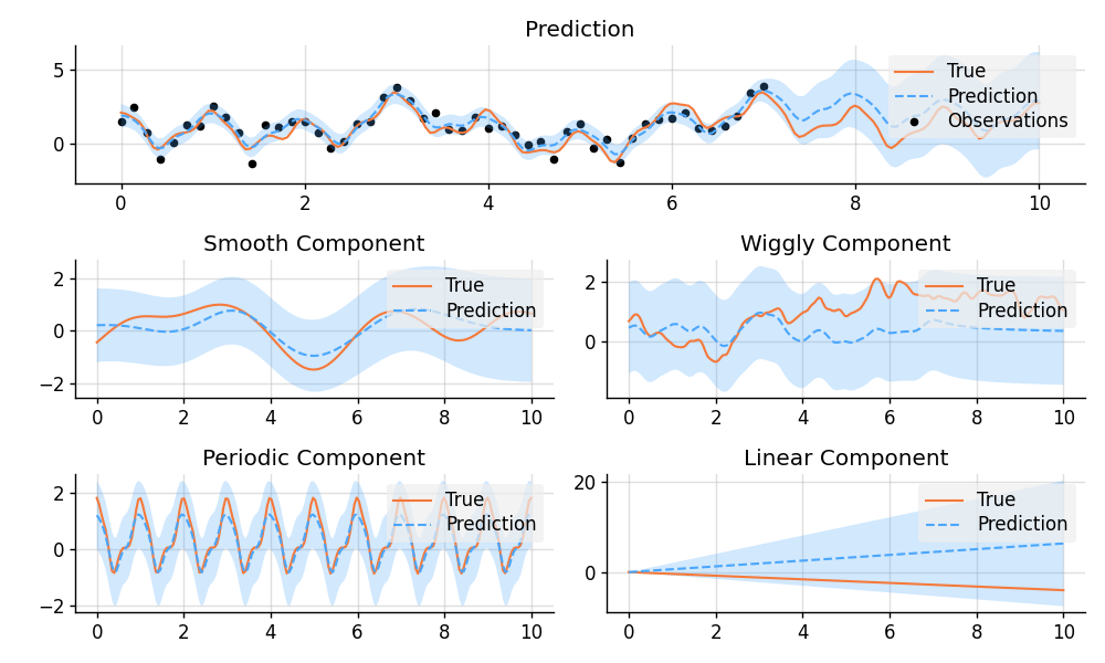 + +```python +import matplotlib.pyplot as plt +from wbml.plot import tweak + +from stheno import Measure, GP, EQ, RQ, Linear, Delta, Exp, B + +B.epsilon = 1e-10 + +# Define points to predict at. +x = B.linspace(0, 10, 200) +x_obs = B.linspace(0, 7, 50) + + +with Measure() as prior: + # Construct a latent function consisting of four different components. + f_smooth = GP(EQ()) + f_wiggly = GP(RQ(1e-1).stretch(0.5)) + f_periodic = GP(EQ().periodic(1.0)) + f_linear = GP(Linear()) + f = f_smooth + f_wiggly + f_periodic + 0.2 * f_linear + + # Let the observation noise consist of a bit of exponential noise. + e_indep = GP(Delta()) + e_exp = GP(Exp()) + e = e_indep + 0.3 * e_exp + + # Sum the latent function and observation noise to get a model for the observations. + y = f + 0.5 * e + +# Sample a true, underlying function and observations. +( + f_true_smooth, + f_true_wiggly, + f_true_periodic, + f_true_linear, + f_true, + y_obs, +) = prior.sample(f_smooth(x), f_wiggly(x), f_periodic(x), f_linear(x), f(x), y(x_obs)) + +# Now condition on the observations and make predictions for the latent function and +# its various components. +post = prior | (y(x_obs), y_obs) + +pred_smooth = post(f_smooth(x)) +pred_wiggly = post(f_wiggly(x)) +pred_periodic = post(f_periodic(x)) +pred_linear = post(f_linear(x)) +pred_f = post(f(x)) + + +# Plot results. +def plot_prediction(x, f, pred, x_obs=None, y_obs=None): + plt.plot(x, f, label="True", style="test") + if x_obs is not None: + plt.scatter(x_obs, y_obs, label="Observations", style="train", s=20) + mean, lower, upper = pred.marginal_credible_bounds() + plt.plot(x, mean, label="Prediction", style="pred") + plt.fill_between(x, lower, upper, style="pred") + tweak() + + +plt.figure(figsize=(10, 6)) + +plt.subplot(3, 1, 1) +plt.title("Prediction") +plot_prediction(x, f_true, pred_f, x_obs, y_obs) + +plt.subplot(3, 2, 3) +plt.title("Smooth Component") +plot_prediction(x, f_true_smooth, pred_smooth) + +plt.subplot(3, 2, 4) +plt.title("Wiggly Component") +plot_prediction(x, f_true_wiggly, pred_wiggly) + +plt.subplot(3, 2, 5) +plt.title("Periodic Component") +plot_prediction(x, f_true_periodic, pred_periodic) + +plt.subplot(3, 2, 6) +plt.title("Linear Component") +plot_prediction(x, f_true_linear, pred_linear) + +plt.savefig("readme_example2_decomposition.png") +plt.show() +``` + +### Learn a Function, Incorporating Prior Knowledge About Its Form + +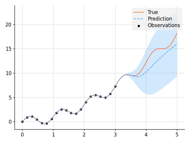 + +```python +import matplotlib.pyplot as plt +import tensorflow as tf +import wbml.out as out +from varz.spec import parametrised, Positive +from varz.tensorflow import Vars, minimise_l_bfgs_b +from wbml.plot import tweak + +from stheno.tensorflow import B, Measure, GP, EQ, Delta + +# Define points to predict at. +x = B.linspace(tf.float64, 0, 5, 100) +x_obs = B.linspace(tf.float64, 0, 3, 20) + + +@parametrised +def model( + vs, + u_var: Positive = 0.5, + u_scale: Positive = 0.5, + noise: Positive = 0.5, + alpha: Positive = 1.2, +): + with Measure(): + # Random fluctuation: + u = GP(u_var * EQ().stretch(u_scale)) + # Construct model. + f = u + (lambda x: x**alpha) + return f, noise + + +# Sample a true, underlying function and observations. +vs = Vars(tf.float64) +f_true = x**1.8 + B.sin(2 * B.pi * x) +f, y = model(vs) +post = f.measure | (f(x), f_true) +y_obs = post(f(x_obs)).sample() + + +def objective(vs): + f, noise = model(vs) + evidence = f(x_obs, noise).logpdf(y_obs) + return -evidence + + +# Learn hyperparameters. +minimise_l_bfgs_b(objective, vs, jit=True) +f, noise = model(vs) + +# Print the learned parameters. +out.kv("Prior", f.display(out.format)) +vs.print() + +# Condition on the observations to make predictions. +f_post = f | (f(x_obs, noise), y_obs) +mean, lower, upper = f_post(x).marginal_credible_bounds() + +# Plot result. +plt.plot(x, B.squeeze(f_true), label="True", style="test") +plt.scatter(x_obs, B.squeeze(y_obs), label="Observations", style="train", s=20) +plt.plot(x, mean, label="Prediction", style="pred") +plt.fill_between(x, lower, upper, style="pred") +tweak() + +plt.savefig("readme_example3_parametric.png") +plt.show() +``` + +### Multi-Output Regression + +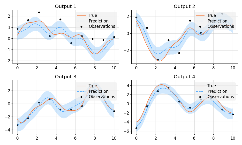 + +```python +import matplotlib.pyplot as plt +from wbml.plot import tweak + +from stheno import B, Measure, GP, EQ, Delta + + +class VGP: + """A vector-valued GP.""" + + def __init__(self, ps): + self.ps = ps + + def __add__(self, other): + return VGP([f + g for f, g in zip(self.ps, other.ps)]) + + def lmatmul(self, A): + m, n = A.shape + ps = [0 for _ in range(m)] + for i in range(m): + for j in range(n): + ps[i] += A[i, j] * self.ps[j] + return VGP(ps) + + +# Define points to predict at. +x = B.linspace(0, 10, 100) +x_obs = B.linspace(0, 10, 10) + +# Model parameters: +m = 2 +p = 4 +H = B.randn(p, m) + + +with Measure() as prior: + # Construct latent functions. + us = VGP([GP(EQ()) for _ in range(m)]) + + # Construct multi-output prior. + fs = us.lmatmul(H) + + # Construct noise. + e = VGP([GP(0.5 * Delta()) for _ in range(p)]) + + # Construct observation model. + ys = e + fs + +# Sample a true, underlying function and observations. +samples = prior.sample(*(p(x) for p in fs.ps), *(p(x_obs) for p in ys.ps)) +fs_true, ys_obs = samples[:p], samples[p:] + +# Compute the posterior and make predictions. +post = prior.condition(*((p(x_obs), y_obs) for p, y_obs in zip(ys.ps, ys_obs))) +preds = [post(p(x)) for p in fs.ps] + + +# Plot results. +def plot_prediction(x, f, pred, x_obs=None, y_obs=None): + plt.plot(x, f, label="True", style="test") + if x_obs is not None: + plt.scatter(x_obs, y_obs, label="Observations", style="train", s=20) + mean, lower, upper = pred.marginal_credible_bounds() + plt.plot(x, mean, label="Prediction", style="pred") + plt.fill_between(x, lower, upper, style="pred") + tweak() + + +plt.figure(figsize=(10, 6)) +for i in range(4): + plt.subplot(2, 2, i + 1) + plt.title(f"Output {i + 1}") + plot_prediction(x, fs_true[i], preds[i], x_obs, ys_obs[i]) +plt.savefig("readme_example4_multi-output.png") +plt.show() +``` + +### Approximate Integration + +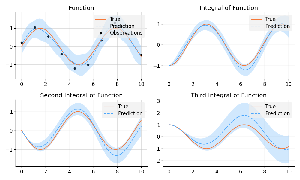 + +```python +import matplotlib.pyplot as plt +import numpy as np +import tensorflow as tf +import wbml.plot + +from stheno.tensorflow import B, Measure, GP, EQ, Delta + +# Define points to predict at. +x = B.linspace(tf.float64, 0, 10, 200) +x_obs = B.linspace(tf.float64, 0, 10, 10) + +with Measure() as prior: + # Construct a model. + f = 0.7 * GP(EQ()).stretch(1.5) + e = 0.2 * GP(Delta()) + + # Construct derivatives. + df = f.diff() + ddf = df.diff() + dddf = ddf.diff() + e + +# Fix the integration constants. +zero = B.cast(tf.float64, 0) +one = B.cast(tf.float64, 1) +prior = prior | ((f(zero), one), (df(zero), zero), (ddf(zero), -one)) + +# Sample observations. +y_obs = B.sin(x_obs) + 0.2 * B.randn(*x_obs.shape) + +# Condition on the observations to make predictions. +post = prior | (dddf(x_obs), y_obs) + +# And make predictions. +pred_iiif = post(f)(x) +pred_iif = post(df)(x) +pred_if = post(ddf)(x) +pred_f = post(dddf)(x) + + +# Plot result. +def plot_prediction(x, f, pred, x_obs=None, y_obs=None): + plt.plot(x, f, label="True", style="test") + if x_obs is not None: + plt.scatter(x_obs, y_obs, label="Observations", style="train", s=20) + mean, lower, upper = pred.marginal_credible_bounds() + plt.plot(x, mean, label="Prediction", style="pred") + plt.fill_between(x, lower, upper, style="pred") + wbml.plot.tweak() + + +plt.figure(figsize=(10, 6)) + +plt.subplot(2, 2, 1) +plt.title("Function") +plot_prediction(x, np.sin(x), pred_f, x_obs=x_obs, y_obs=y_obs) + +plt.subplot(2, 2, 2) +plt.title("Integral of Function") +plot_prediction(x, -np.cos(x), pred_if) + +plt.subplot(2, 2, 3) +plt.title("Second Integral of Function") +plot_prediction(x, -np.sin(x), pred_iif) + +plt.subplot(2, 2, 4) +plt.title("Third Integral of Function") +plot_prediction(x, np.cos(x), pred_iiif) + +plt.savefig("readme_example5_integration.png") +plt.show() +``` + +### Bayesian Linear Regression + +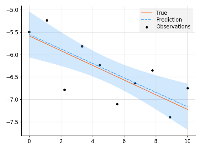 + +```python +import matplotlib.pyplot as plt +import wbml.out as out +from wbml.plot import tweak + +from stheno import B, Measure, GP + +B.epsilon = 1e-10 # Very slightly regularise. + +# Define points to predict at. +x = B.linspace(0, 10, 200) +x_obs = B.linspace(0, 10, 10) + +with Measure() as prior: + # Construct a linear model. + slope = GP(1) + intercept = GP(5) + f = slope * (lambda x: x) + intercept + +# Sample a slope, intercept, underlying function, and observations. +true_slope, true_intercept, f_true, y_obs = prior.sample( + slope(0), intercept(0), f(x), f(x_obs, 0.2) +) + +# Condition on the observations to make predictions. +post = prior | (f(x_obs, 0.2), y_obs) +mean, lower, upper = post(f(x)).marginal_credible_bounds() + +out.kv("True slope", true_slope[0, 0]) +out.kv("Predicted slope", post(slope(0)).mean[0, 0]) +out.kv("True intercept", true_intercept[0, 0]) +out.kv("Predicted intercept", post(intercept(0)).mean[0, 0]) + +# Plot result. +plt.plot(x, f_true, label="True", style="test") +plt.scatter(x_obs, y_obs, label="Observations", style="train", s=20) +plt.plot(x, mean, label="Prediction", style="pred") +plt.fill_between(x, lower, upper, style="pred") +tweak() + +plt.savefig("readme_example6_blr.png") +plt.show() +``` + +### GPAR + +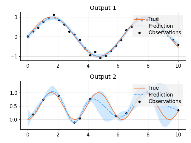 + +```python +import matplotlib.pyplot as plt +import numpy as np +import tensorflow as tf +from varz.spec import parametrised, Positive +from varz.tensorflow import Vars, minimise_l_bfgs_b +from wbml.plot import tweak + +from stheno.tensorflow import B, GP, EQ + +# Define points to predict at. +x = B.linspace(tf.float64, 0, 10, 200) +x_obs1 = B.linspace(tf.float64, 0, 10, 30) +inds2 = np.random.permutation(len(x_obs1))[:10] +x_obs2 = B.take(x_obs1, inds2) + +# Construction functions to predict and observations. +f1_true = B.sin(x) +f2_true = B.sin(x) ** 2 + +y1_obs = B.sin(x_obs1) + 0.1 * B.randn(*x_obs1.shape) +y2_obs = B.sin(x_obs2) ** 2 + 0.1 * B.randn(*x_obs2.shape) + + +@parametrised +def model( + vs, + var1: Positive = 1, + scale1: Positive = 1, + noise1: Positive = 0.1, + var2: Positive = 1, + scale2: Positive = 1, + noise2: Positive = 0.1, +): + # Build layers: + f1 = GP(var1 * EQ().stretch(scale1)) + f2 = GP(var2 * EQ().stretch(scale2)) + return (f1, noise1), (f2, noise2) + + +def objective(vs): + (f1, noise1), (f2, noise2) = model(vs) + x1 = x_obs1 + x2 = B.stack(x_obs2, B.take(y1_obs, inds2), axis=1) + evidence = f1(x1, noise1).logpdf(y1_obs) + f2(x2, noise2).logpdf(y2_obs) + return -evidence + + +# Learn hyperparameters. +vs = Vars(tf.float64) +minimise_l_bfgs_b(objective, vs) + +# Compute posteriors. +(f1, noise1), (f2, noise2) = model(vs) +x1 = x_obs1 +x2 = B.stack(x_obs2, B.take(y1_obs, inds2), axis=1) +f1_post = f1 | (f1(x1, noise1), y1_obs) +f2_post = f2 | (f2(x2, noise2), y2_obs) + +# Predict first output. +mean1, lower1, upper1 = f1_post(x).marginal_credible_bounds() + +# Predict second output with Monte Carlo. +samples = [ + f2_post(B.stack(x, f1_post(x).sample()[:, 0], axis=1)).sample()[:, 0] + for _ in range(100) +] +mean2 = np.mean(samples, axis=0) +lower2 = np.percentile(samples, 2.5, axis=0) +upper2 = np.percentile(samples, 100 - 2.5, axis=0) + +# Plot result. +plt.figure() + +plt.subplot(2, 1, 1) +plt.title("Output 1") +plt.plot(x, f1_true, label="True", style="test") +plt.scatter(x_obs1, y1_obs, label="Observations", style="train", s=20) +plt.plot(x, mean1, label="Prediction", style="pred") +plt.fill_between(x, lower1, upper1, style="pred") +tweak() + +plt.subplot(2, 1, 2) +plt.title("Output 2") +plt.plot(x, f2_true, label="True", style="test") +plt.scatter(x_obs2, y2_obs, label="Observations", style="train", s=20) +plt.plot(x, mean2, label="Prediction", style="pred") +plt.fill_between(x, lower2, upper2, style="pred") +tweak() + +plt.savefig("readme_example7_gpar.png") +plt.show() +``` + +### A GP-RNN Model + +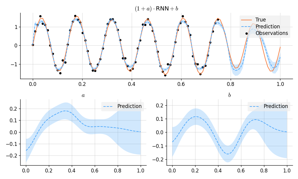 + +```python +import matplotlib.pyplot as plt +import numpy as np +import tensorflow as tf +from varz.spec import parametrised, Positive +from varz.tensorflow import Vars, minimise_adam +from wbml.net import rnn as rnn_constructor +from wbml.plot import tweak + +from stheno.tensorflow import B, Measure, GP, EQ + +# Increase regularisation because we are dealing with `tf.float32`s. +B.epsilon = 1e-6 + +# Construct points which to predict at. +x = B.linspace(tf.float32, 0, 1, 100)[:, None] +inds_obs = B.range(0, int(0.75 * len(x))) # Train on the first 75% only. +x_obs = B.take(x, inds_obs) + +# Construct function and observations. +# Draw random modulation functions. +a_true = GP(1e-2 * EQ().stretch(0.1))(x).sample() +b_true = GP(1e-2 * EQ().stretch(0.1))(x).sample() +# Construct the true, underlying function. +f_true = (1 + a_true) * B.sin(2 * np.pi * 7 * x) + b_true +# Add noise. +y_true = f_true + 0.1 * B.randn(*f_true.shape) + +# Normalise and split. +f_true = (f_true - B.mean(y_true)) / B.std(y_true) +y_true = (y_true - B.mean(y_true)) / B.std(y_true) +y_obs = B.take(y_true, inds_obs) + + +@parametrised +def model(vs, a_scale: Positive = 0.1, b_scale: Positive = 0.1, noise: Positive = 0.01): + # Construct an RNN. + f_rnn = rnn_constructor( + output_size=1, widths=(10,), nonlinearity=B.tanh, final_dense=True + ) + + # Set the weights for the RNN. + num_weights = f_rnn.num_weights(input_size=1) + weights = Vars(tf.float32, source=vs.get(shape=(num_weights,), name="rnn")) + f_rnn.initialise(input_size=1, vs=weights) + + with Measure(): + # Construct GPs that modulate the RNN. + a = GP(1e-2 * EQ().stretch(a_scale)) + b = GP(1e-2 * EQ().stretch(b_scale)) + + # GP-RNN model: + f_gp_rnn = (1 + a) * (lambda x: f_rnn(x)) + b + + return f_rnn, f_gp_rnn, noise, a, b + + +def objective_rnn(vs): + f_rnn, _, _, _, _ = model(vs) + return B.mean((f_rnn(x_obs) - y_obs) ** 2) + + +def objective_gp_rnn(vs): + _, f_gp_rnn, noise, _, _ = model(vs) + evidence = f_gp_rnn(x_obs, noise).logpdf(y_obs) + return -evidence + + +# Pretrain the RNN. +vs = Vars(tf.float32) +minimise_adam(objective_rnn, vs, rate=5e-3, iters=1000, trace=True, jit=True) + +# Jointly train the RNN and GPs. +minimise_adam(objective_gp_rnn, vs, rate=1e-3, iters=1000, trace=True, jit=True) + +_, f_gp_rnn, noise, a, b = model(vs) + +# Condition. +post = f_gp_rnn.measure | (f_gp_rnn(x_obs, noise), y_obs) + +# Predict and plot results. +plt.figure(figsize=(10, 6)) + +plt.subplot(2, 1, 1) +plt.title("$(1 + a)\\cdot {}$RNN${} + b$") +plt.plot(x, f_true, label="True", style="test") +plt.scatter(x_obs, y_obs, label="Observations", style="train", s=20) +mean, lower, upper = post(f_gp_rnn(x)).marginal_credible_bounds() +plt.plot(x, mean, label="Prediction", style="pred") +plt.fill_between(x, lower, upper, style="pred") +tweak() + +plt.subplot(2, 2, 3) +plt.title("$a$") +mean, lower, upper = post(a(x)).marginal_credible_bounds() +plt.plot(x, mean, label="Prediction", style="pred") +plt.fill_between(x, lower, upper, style="pred") +tweak() + +plt.subplot(2, 2, 4) +plt.title("$b$") +mean, lower, upper = post(b(x)).marginal_credible_bounds() +plt.plot(x, mean, label="Prediction", style="pred") +plt.fill_between(x, lower, upper, style="pred") +tweak() + +plt.savefig(f"readme_example8_gp-rnn.png") +plt.show() +``` + +### Approximate Multiplication Between GPs + +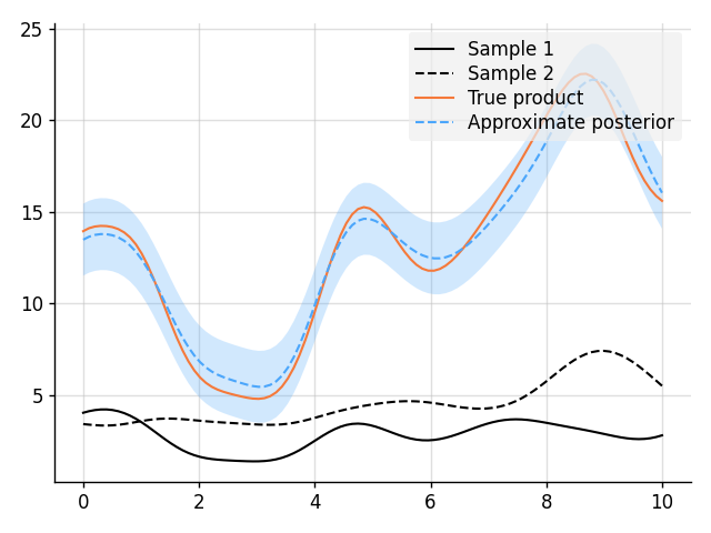 + +```python +import matplotlib.pyplot as plt +from wbml.plot import tweak + +from stheno import B, Measure, GP, EQ + +# Define points to predict at. +x = B.linspace(0, 10, 100) + +with Measure() as prior: + f1 = GP(3, EQ()) + f2 = GP(3, EQ()) + + # Compute the approximate product. + f_prod = f1 * f2 + +# Sample two functions. +s1, s2 = prior.sample(f1(x), f2(x)) + +# Predict. +f_prod_post = f_prod | ((f1(x), s1), (f2(x), s2)) +mean, lower, upper = f_prod_post(x).marginal_credible_bounds() + +# Plot result. +plt.plot(x, s1, label="Sample 1", style="train") +plt.plot(x, s2, label="Sample 2", style="train", ls="--") +plt.plot(x, s1 * s2, label="True product", style="test") +plt.plot(x, mean, label="Approximate posterior", style="pred") +plt.fill_between(x, lower, upper, style="pred") +tweak() + +plt.savefig("readme_example9_product.png") +plt.show() +``` + +### Sparse Regression + +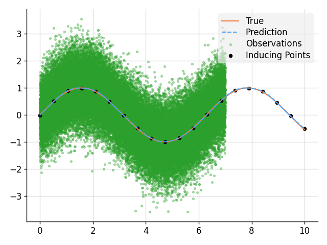 + +```python +import matplotlib.pyplot as plt +import wbml.out as out +from wbml.plot import tweak + +from stheno import B, GP, EQ, PseudoObs + +# Define points to predict at. +x = B.linspace(0, 10, 100) +x_obs = B.linspace(0, 7, 50_000) +x_ind = B.linspace(0, 10, 20) + +# Construct a prior. +f = GP(EQ().periodic(2 * B.pi)) + +# Sample a true, underlying function and observations. +f_true = B.sin(x) +y_obs = B.sin(x_obs) + B.sqrt(0.5) * B.randn(*x_obs.shape) + +# Compute a pseudo-point approximation of the posterior. +obs = PseudoObs(f(x_ind), (f(x_obs, 0.5), y_obs)) + +# Compute the ELBO. +out.kv("ELBO", obs.elbo(f.measure)) + +# Compute the approximate posterior. +f_post = f | obs + +# Make predictions with the approximate posterior. +mean, lower, upper = f_post(x).marginal_credible_bounds() + +# Plot result. +plt.plot(x, f_true, label="True", style="test") +plt.scatter( + x_obs, + y_obs, + label="Observations", + style="train", + c="tab:green", + alpha=0.35, +) +plt.scatter( + x_ind, + obs.mu(f.measure)[:, 0], + label="Inducing Points", + style="train", + s=20, +) +plt.plot(x, mean, label="Prediction", style="pred") +plt.fill_between(x, lower, upper, style="pred") +tweak() + +plt.savefig("readme_example10_sparse.png") +plt.show() +``` + +### Smoothing with Nonparametric Basis Functions + +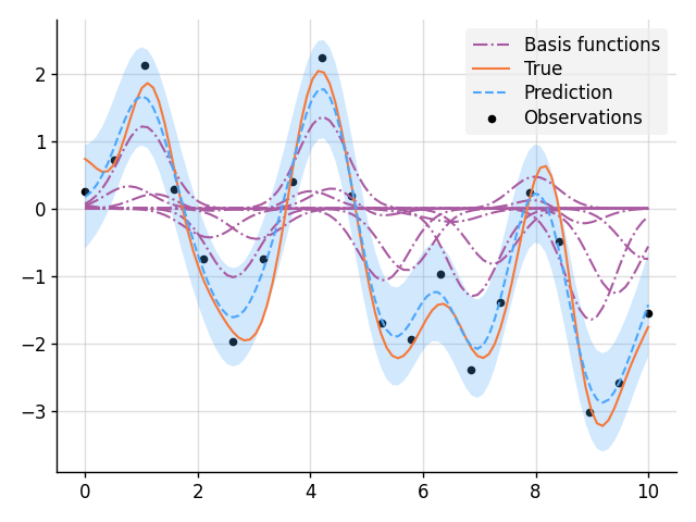 + +```python +import matplotlib.pyplot as plt +from wbml.plot import tweak + +from stheno import B, Measure, GP, EQ + +# Define points to predict at. +x = B.linspace(0, 10, 100) +x_obs = B.linspace(0, 10, 20) + +with Measure() as prior: + w = lambda x: B.exp(-(x**2) / 0.5) # Basis function + b = [(w * GP(EQ())).shift(xi) for xi in x_obs] # Weighted basis functions + f = sum(b) + +# Sample a true, underlying function and observations. +f_true, y_obs = prior.sample(f(x), f(x_obs, 0.2)) + +# Condition on the observations to make predictions. +post = prior | (f(x_obs, 0.2), y_obs) + +# Plot result. +for i, bi in enumerate(b): + mean, lower, upper = post(bi(x)).marginal_credible_bounds() + kw_args = {"label": "Basis functions"} if i == 0 else {} + plt.plot(x, mean, style="pred2", **kw_args) +plt.plot(x, f_true, label="True", style="test") +plt.scatter(x_obs, y_obs, label="Observations", style="train", s=20) +mean, lower, upper = post(f(x)).marginal_credible_bounds() +plt.plot(x, mean, label="Prediction", style="pred") +plt.fill_between(x, lower, upper, style="pred") +tweak() + +plt.savefig("readme_example11_nonparametric_basis.png") +plt.show() +``` + + + +%package -n python3-stheno +Summary: Implementation of Gaussian processes in Python +Provides: python-stheno +BuildRequires: python3-devel +BuildRequires: python3-setuptools +BuildRequires: python3-pip +%description -n python3-stheno +# [Stheno](https://github.com/wesselb/stheno) + +[](https://github.com/wesselb/stheno/actions?query=workflow%3ACI) +[](https://coveralls.io/github/wesselb/stheno?branch=master) +[](https://wesselb.github.io/stheno) +[](https://github.com/psf/black) + +Stheno is an implementation of Gaussian process modelling in Python. See +also [Stheno.jl](https://github.com/willtebbutt/Stheno.jl). + +[Check out our post about linear models with Stheno and JAX.](https://wesselb.github.io/2021/01/19/linear-models-with-stheno-and-jax.html) + +Contents: + +* [Nonlinear Regression in 20 Seconds](#nonlinear-regression-in-20-seconds) +* [Installation](#installation) +* [Manual](#manual) + - [AutoGrad, TensorFlow, PyTorch, or JAX? Your Choice!](#autograd-tensorflow-pytorch-or-jax-your-choice) + - [Model Design](#model-design) + - [Finite-Dimensional Distributions](#finite-dimensional-distributions) + - [Prior and Posterior Measures](#prior-and-posterior-measures) + - [Inducing Points](#inducing-points) + - [Kernels and Means](#kernels-and-means) + - [Batched Computation](#batched-computation) + - [Important Remarks](#important-remarks) +* [Examples](#examples) + - [Simple Regression](#simple-regression) + - [Hyperparameter Optimisation with Varz](#hyperparameter-optimisation-with-varz) + - [Hyperparameter Optimisation with PyTorch](#hyperparameter-optimisation-with-pytorch) + - [Decomposition of Prediction](#decomposition-of-prediction) + - [Learn a Function, Incorporating Prior Knowledge About Its Form](#learn-a-function-incorporating-prior-knowledge-about-its-form) + - [Multi-Output Regression](#multi-output-regression) + - [Approximate Integration](#approximate-integration) + - [Bayesian Linear Regression](#bayesian-linear-regression) + - [GPAR](#gpar) + - [A GP-RNN Model](#a-gp-rnn-model) + - [Approximate Multiplication Between GPs](#approximate-multiplication-between-gps) + - [Sparse Regression](#sparse-regression) + - [Smoothing with Nonparametric Basis Functions](#smoothing-with-nonparametric-basis-functions) + +## Nonlinear Regression in 20 Seconds + +```python +>>> import numpy as np + +>>> from stheno import GP, EQ + +>>> x = np.linspace(0, 2, 10) # Some points to predict at + +>>> y = x ** 2 # Some observations + +>>> f = GP(EQ()) # Construct Gaussian process. + +>>> f_post = f | (f(x), y) # Compute the posterior. + +>>> pred = f_post(np.array([1, 2, 3])) # Predict! + +>>> pred.mean +<dense matrix: shape=3x1, dtype=float64 + mat=[[1. ] + [4. ] + [8.483]]> + +>>> pred.var +<dense matrix: shape=3x3, dtype=float64 + mat=[[ 8.032e-13 7.772e-16 -4.577e-09] + [ 7.772e-16 9.999e-13 2.773e-10] + [-4.577e-09 2.773e-10 3.313e-03]]> +``` + +[These custom matrix types are there to accelerate the underlying linear algebra.](#important-remarks) +To get vanilla NumPy/AutoGrad/TensorFlow/PyTorch/JAX arrays, use `B.dense`: + +```python +>>> from lab import B + +>>> B.dense(pred.mean) +array([[1.00000068], + [3.99999999], + [8.4825932 ]]) + +>>> B.dense(pred.var) +array([[ 8.03246358e-13, 7.77156117e-16, -4.57690943e-09], + [ 7.77156117e-16, 9.99866856e-13, 2.77333267e-10], + [-4.57690943e-09, 2.77333267e-10, 3.31283378e-03]]) +``` + +Moar?! Then read on! + +## Installation + +See [the instructions here](https://gist.github.com/wesselb/4b44bf87f3789425f96e26c4308d0adc). +Then simply + +``` +pip install stheno +``` + +## Manual + +Note: [here](https://wesselb.github.io/stheno) is a nicely rendered and more +readable version of the docs. + +### AutoGrad, TensorFlow, PyTorch, or JAX? Your Choice! + +```python +from stheno.autograd import GP, EQ +``` + +```python +from stheno.tensorflow import GP, EQ +``` + +```python +from stheno.torch import GP, EQ +``` + +```python +from stheno.jax import GP, EQ +``` + +### Model Design + +The basic building block is a `f = GP(mean=0, kernel, measure=prior)`, which takes +in [a _mean_, a _kernel_](#kernels-and-means), and a _measure_. +The mean and kernel of a GP can be extracted with `f.mean` and `f.kernel`. +The measure should be thought of as a big joint distribution that assigns a mean and +a kernel to every variable `f`. +A measure can be created with `prior = Measure()`. +A GP `f` can have different means and kernels under different measures. +For example, under some _prior_ measure, `f` can have an `EQ()` kernel; but, under some +_posterior_ measure, `f` has a kernel that is determined by the posterior distribution +of a GP. +[We will see later how posterior measures can be constructed.](#prior-and-posterior-measures) +The measure with which a `f = GP(kernel, measure=prior)` is constructed can be +extracted with `f.measure == prior`. +If the keyword argument `measure` is not set, then automatically a new measure is +created, which afterwards can be extracted with `f.measure`. + +Definition, where `prior = Measure()`: + +```python +f = GP(kernel) + +f = GP(mean, kernel) + +f = GP(kernel, measure=prior) + +f = GP(mean, kernel, measure=prior) +``` + +GPs that are associated to the same measure can be combined into new GPs, which is +the primary mechanism used to build cool models. + +Here's an example model: + +```python +>>> prior = Measure() + +>>> f1 = GP(lambda x: x ** 2, EQ(), measure=prior) + +>>> f1 +GP(<lambda>, EQ()) + +>>> f2 = GP(Linear(), measure=prior) + +>>> f2 +GP(0, Linear()) + +>>> f_sum = f1 + f2 + +>>> f_sum +GP(<lambda>, EQ() + Linear()) + +>>> f_sum + GP(EQ()) # Not valid: `GP(EQ())` belongs to a new measure! +AssertionError: Processes GP(<lambda>, EQ() + Linear()) and GP(0, EQ()) are associated to different measures. +``` + +To avoid setting the keyword `measure` for every `GP` that you create, you can enter +a measure as a context: + +```python +>>> with Measure() as prior: + f1 = GP(lambda x: x ** 2, EQ()) + f2 = GP(Linear()) + f_sum = f1 + f2 + +>>> prior == f1.measure == f2.measure == f_sum.measure +True +``` + + + +#### Compositional Design + +* Add and subtract GPs and other objects. + + Example: + + ```python + >>> GP(EQ(), measure=prior) + GP(Exp(), measure=prior) + GP(0, EQ() + Exp()) + + >>> GP(EQ(), measure=prior) + GP(EQ(), measure=prior) + GP(0, 2 * EQ()) + + >>> GP(EQ()) + 1 + GP(1, EQ()) + + >>> GP(EQ()) + 0 + GP(0, EQ()) + + >>> GP(EQ()) + (lambda x: x ** 2) + GP(<lambda>, EQ()) + + >>> GP(2, EQ(), measure=prior) - GP(1, EQ(), measure=prior) + GP(1, 2 * EQ()) + ``` + +* Multiply GPs and other objects. + + *Warning:* + The product of two GPs it *not* a Gaussian process. + Stheno approximates the resulting process by moment matching. + + Example: + + ```python + >>> GP(1, EQ(), measure=prior) * GP(1, Exp(), measure=prior) + GP(<lambda> + <lambda> + -1 * 1, <lambda> * Exp() + <lambda> * EQ() + EQ() * Exp()) + + >>> 2 * GP(EQ()) + GP(2, 2 * EQ()) + + >>> 0 * GP(EQ()) + GP(0, 0) + + >>> (lambda x: x) * GP(EQ()) + GP(0, <lambda> * EQ()) + ``` + +* Shift GPs. + + Example: + + ```python + >>> GP(EQ()).shift(1) + GP(0, EQ() shift 1) + ``` + +* Stretch GPs. + + Example: + + ```python + >>> GP(EQ()).stretch(2) + GP(0, EQ() > 2) + ``` + +* Select particular input dimensions. + + Example: + + ```python + >>> GP(EQ()).select(1, 3) + GP(0, EQ() : [1, 3]) + ``` + +* Transform the input. + + Example: + + ```python + >>> GP(EQ()).transform(f) + GP(0, EQ() transform f) + ``` + +* Numerically take the derivative of a GP. + The argument specifies which dimension to take the derivative with respect + to. + + Example: + + ```python + >>> GP(EQ()).diff(1) + GP(0, d(1) EQ()) + ``` + +* Construct a finite difference estimate of the derivative of a GP. + See `Measure.diff_approx` for a description of the arguments. + + Example: + + ```python + >>> GP(EQ()).diff_approx(deriv=1, order=2) + GP(50000000.0 * (0.5 * EQ() + 0.5 * ((-0.5 * (EQ() shift (0.0001414213562373095, 0))) shift (0, -0.0001414213562373095)) + 0.5 * ((-0.5 * (EQ() shift (0, 0.0001414213562373095))) shift (-0.0001414213562373095, 0))), 0) + ``` + +* Construct the Cartesian product of a collection of GPs. + + Example: + + ```python + >>> prior = Measure() + + >>> f1, f2 = GP(EQ(), measure=prior), GP(EQ(), measure=prior) + + >>> cross(f1, f2) + GP(MultiOutputMean(0, 0), MultiOutputKernel(EQ(), EQ())) + ``` + +#### Displaying GPs + +GPs have a `display` method that accepts a formatter. + +Example: + +```python +>>> print(GP(2.12345 * EQ()).display(lambda x: f"{x:.2f}")) +GP(2.12 * EQ(), 0) +``` + +#### Properties of GPs + +[Properties of kernels](https://github.com/wesselb/mlkernels#properties-of-kernels-and-means) +can be queried on GPs directly. + +Example: + +```python +>>> GP(EQ()).stationary +True +``` + +#### Naming GPs + +It is possible to give a name to a GP. +Names must be strings. +A measure then behaves like a two-way dictionary between GPs and their names. + +Example: + +```python +>>> prior = Measure() + +>>> p = GP(EQ(), name="name", measure=prior) + +>>> p.name +'name' + +>>> p.name = "alternative_name" + +>>> prior["alternative_name"] +GP(0, EQ()) + +>>> prior[p] +'alternative_name' +``` + +### Finite-Dimensional Distributions + +Simply call a GP to construct a finite-dimensional distribution at some inputs. +You can give a second argument, which specifies the variance of additional additive +noise. +After constructing a finite-dimensional distribution, you can compute the mean, +the variance, sample, or compute a logpdf. + +Definition, where `f` is a `GP`: + +```python +f(x) # No additional noise + +f(x, noise) # Additional noise with variance `noise` +``` + +Things you can do with a finite-dimensional distribution: + +* + Use `f(x).mean` to compute the mean. + +* + Use `f(x).var` to compute the variance. + +* + Use `f(x).mean_var` to compute simultaneously compute the mean and variance. + This can be substantially more efficient than calling first `f(x).mean` and then + `f(x).var`. + +* + Use `Normal.sample` to sample. + + Definition: + + ```python + f(x).sample() # Produce one sample. + + f(x).sample(n) # Produce `n` samples. + + f(x).sample(noise=noise) # Produce one samples with additional noise variance `noise`. + + f(x).sample(n, noise=noise) # Produce `n` samples with additional noise variance `noise`. + ``` + +* + Use `f(x).logpdf(y)` to compute the logpdf of some data `y`. + +* + Use `means, variances = f(x).marginals()` to efficiently compute the marginal means + and marginal variances. + + Example: + + ```python + >>> f(x).marginals() + (array([0., 0., 0.]), np.array([1., 1., 1.])) + ``` + +* + Use `means, lowers, uppers = f(x).marginal_credible_bounds()` to efficiently compute + the means and the marginal lower and upper 95% central credible region bounds. + + Example: + + ```python + >>> f(x).marginal_credible_bounds() + (array([0., 0., 0.]), array([-1.96, -1.96, -1.96]), array([1.96, 1.96, 1.96])) + ``` + +* + Use `Measure.logpdf` to compute the joint logpdf of multiple observations. + + Definition, where `prior = Measure()`: + + ```python + prior.logpdf(f(x), y) + + prior.logpdf((f1(x1), y1), (f2(x2), y2), ...) + ``` + +* + Use `Measure.sample` to jointly sample multiple observations. + + Definition, where `prior = Measure()`: + + ```python + sample = prior.sample(f(x)) + + sample1, sample2, ... = prior.sample(f1(x1), f2(x2), ...) + ``` + +Example: + +```python +>>> prior = Measure() + +>>> f = GP(EQ(), measure=prior) + +>>> x = np.array([0., 1., 2.]) + +>>> f(x) # FDD without noise. +<FDD: + process=GP(0, EQ()), + input=array([0., 1., 2.]), + noise=<zero matrix: shape=3x3, dtype=float64> + +>>> f(x, 0.1) # FDD with noise. +<FDD: + process=GP(0, EQ()), + input=array([0., 1., 2.]), + noise=<diagonal matrix: shape=3x3, dtype=float64 + diag=[0.1 0.1 0.1]>> + +>>> f(x).mean +array([[0.], + [0.], + [0.]]) + +>>> f(x).var +<dense matrix: shape=3x3, dtype=float64 + mat=[[1. 0.607 0.135] + [0.607 1. 0.607] + [0.135 0.607 1. ]]> + +>>> y1 = f(x).sample() + +>>> y1 +array([[-0.45172746], + [ 0.46581948], + [ 0.78929767]]) + +>>> f(x).logpdf(y1) +-2.811609567720761 + +>>> y2 = f(x).sample(2) +array([[-0.43771276, -2.36741858], + [ 0.86080043, -1.22503079], + [ 2.15779126, -0.75319405]] + +>>> f(x).logpdf(y2) + array([-4.82949038, -5.40084225]) +``` + +### Prior and Posterior Measures + +Conditioning a _prior_ measure on observations gives a _posterior_ measure. +To condition a measure on observations, use `Measure.__or__`. + +Definition, where `prior = Measure()` and `f*` are `GP`s: + +```python +post = prior | (f(x, [noise]), y) + +post = prior | ((f1(x1, [noise1]), y1), (f2(x2, [noise2]), y2), ...) +``` + +You can then obtain a posterior process with `post(f)` and a finite-dimensional +distribution under the posterior with `post(f(x))`. +Alternatively, the posterior of a process `f` can be obtained by conditioning `f` +directly. + +Definition, where and `f*` are `GP`s: + +```python +f_post = f | (f(x, [noise]), y) + +f_post = f | ((f1(x1, [noise1]), y1), (f2(x2, [noise2]), y2), ...) +``` + +Let's consider an example. +First, build a model and sample some values. + +```python +>>> prior = Measure() + +>>> f = GP(EQ(), measure=prior) + +>>> x = np.array([0., 1., 2.]) + +>>> y = f(x).sample() +``` + +Then compute the posterior measure. + +```python +>>> post = prior | (f(x), y) + +>>> post(f) +GP(PosteriorMean(), PosteriorKernel()) + +>>> post(f).mean(x) +<dense matrix: shape=3x1, dtype=float64 + mat=[[ 0.412] + [-0.811] + [-0.933]]> + +>>> post(f).kernel(x) +<dense matrix: shape=3x3, dtype=float64 + mat=[[1.e-12 0.e+00 0.e+00] + [0.e+00 1.e-12 0.e+00] + [0.e+00 0.e+00 1.e-12]]> + +>>> post(f(x)) +<FDD: + process=GP(PosteriorMean(), PosteriorKernel()), + input=array([0., 1., 2.]), + noise=<zero matrix: shape=3x3, dtype=float64>> + +>>> post(f(x)).mean +<dense matrix: shape=3x1, dtype=float64 + mat=[[ 0.412] + [-0.811] + [-0.933]]> + +>>> post(f(x)).var +<dense matrix: shape=3x3, dtype=float64 + mat=[[1.e-12 0.e+00 0.e+00] + [0.e+00 1.e-12 0.e+00] + [0.e+00 0.e+00 1.e-12]]> +``` + +We can also obtain the posterior by conditioning `f` directly: + +```python +>>> f_post = f | (f(x), y) + +>>> f_post +GP(PosteriorMean(), PosteriorKernel()) + +>>> f_post.mean(x) +<dense matrix: shape=3x1, dtype=float64 + mat=[[ 0.412] + [-0.811] + [-0.933]]> + +>>> f_post.kernel(x) +<dense matrix: shape=3x3, dtype=float64 + mat=[[1.e-12 0.e+00 0.e+00] + [0.e+00 1.e-12 0.e+00] + [0.e+00 0.e+00 1.e-12]]> + +>>> f_post(x) +<FDD: + process=GP(PosteriorMean(), PosteriorKernel()), + input=array([0., 1., 2.]), + noise=<zero matrix: shape=3x3, dtype=float64>> + +>>> f_post(x).mean +<dense matrix: shape=3x1, dtype=float64 + mat=[[ 0.412] + [-0.811] + [-0.933]]> + +>>> f_post(x).var +<dense matrix: shape=3x3, dtype=float64 + mat=[[1.e-12 0.e+00 0.e+00] + [0.e+00 1.e-12 0.e+00] + [0.e+00 0.e+00 1.e-12]]> +``` + +We can further extend our model by building on the posterior. + +```python +>>> g = GP(Linear(), measure=post) + +>>> f_sum = post(f) + g + +>>> f_sum +GP(PosteriorMean(), PosteriorKernel() + Linear()) +``` + +However, what we cannot do is mixing the prior and posterior. + +```python +>>> f + g +AssertionError: Processes GP(0, EQ()) and GP(0, Linear()) are associated to different measures. +``` + +### Inducing Points + +Stheno supports pseudo-point approximations of posterior distributions with +various approximation methods: + +1. The Variational Free Energy (VFE; + [Titsias, 2009](http://proceedings.mlr.press/v5/titsias09a/titsias09a.pdf)) + approximation. + To use the VFE approximation, use `PseudoObs`. + +2. The Fully Independent Training Conditional (FITC; + [Snelson & Ghahramani, 2006](http://www.gatsby.ucl.ac.uk/~snelson/SPGP_up.pdf)) + approximation. + To use the FITC approximation, use `PseudoObsFITC`. + +3. The Deterministic Training Conditional (DTC; + [Csato & Opper, 2002](https://direct.mit.edu/neco/article/14/3/641/6594/Sparse-On-Line-Gaussian-Processes); + [Seeger et al., 2003](http://proceedings.mlr.press/r4/seeger03a/seeger03a.pdf)) + approximation. + To use the DTC approximation, use `PseudoObsDTC`. + +The VFE approximation (`PseudoObs`) is the approximation recommended to use. +The following definitions and examples will use the VFE approximation with `PseudoObs`, +but every instance of `PseudoObs` can be swapped out for `PseudoObsFITC` or +`PseudoObsDTC`. + +Definition: + +```python +obs = PseudoObs( + u(z), # FDD of inducing points + (f(x, [noise]), y) # Observed data +) + +obs = PseudoObs(u(z), f(x, [noise]), y) + +obs = PseudoObs(u(z), (f1(x1, [noise1]), y1), (f2(x2, [noise2]), y2), ...) + +obs = PseudoObs((u1(z1), u2(z2), ...), f(x, [noise]), y) + +obs = PseudoObs((u1(z1), u2(z2), ...), (f1(x1, [noise1]), y1), (f2(x2, [noise2]), y2), ...) +``` + +The approximate posterior measure can be constructed with `prior | obs` +where `prior = Measure()` is the measure of your model. +To quantify the quality of the approximation, you can compute the ELBO with +`obs.elbo(prior)`. + +Let's consider an example. +First, build a model and sample some noisy observations. + +```python +>>> prior = Measure() + +>>> f = GP(EQ(), measure=prior) + +>>> x_obs = np.linspace(0, 10, 2000) + +>>> y_obs = f(x_obs, 1).sample() +``` + +Ouch, computing the logpdf is quite slow: + +```python +>>> %timeit f(x_obs, 1).logpdf(y_obs) +219 ms ± 35.7 ms per loop (mean ± std. dev. of 7 runs, 10 loops each) +``` + +Let's try to use inducing points to speed this up. + +```python +>>> x_ind = np.linspace(0, 10, 100) + +>>> u = f(x_ind) # FDD of inducing points. + +>>> %timeit PseudoObs(u, f(x_obs, 1), y_obs).elbo(prior) +9.8 ms ± 181 µs per loop (mean ± std. dev. of 7 runs, 100 loops each) +``` + +Much better. +And the approximation is good: + +```python +>>> PseudoObs(u, f(x_obs, 1), y_obs).elbo(prior) - f(x_obs, 1).logpdf(y_obs) +-3.537934389896691e-10 +``` + +We finally construct the approximate posterior measure: + +```python +>>> post_approx = prior | PseudoObs(u, f(x_obs, 1), y_obs) + +>>> post_approx(f(x_obs)).mean +<dense matrix: shape=2000x1, dtype=float64 + mat=[[0.469] + [0.468] + [0.467] + ... + [1.09 ] + [1.09 ] + [1.091]]> +``` + + +### Kernels and Means + +See [MLKernels](https://github.com/wesselb/mlkernels). + + +### Batched Computation + +Stheno supports batched computation. +See [MLKernels](https://github.com/wesselb/mlkernels/#usage) for a description of how +means and kernels work with batched computation. + +Example: + +```python +>>> f = GP(EQ()) + +>>> x = np.random.randn(16, 100, 1) + +>>> y = f(x, 1).sample() + +>>> logpdf = f(x, 1).logpdf(y) + +>>> y.shape +(16, 100, 1) + +>>> f(x, 1).logpdf(y).shape +(16,) +``` + + +### Important Remarks + +Stheno uses [LAB](https://github.com/wesselb/lab) to provide an implementation that is +backend agnostic. +Moreover, Stheno uses [an extension of LAB](https://github.com/wesselb/matrix) to +accelerate linear algebra with structured linear algebra primitives. +You will encounter these primitives: + +```python +>>> k = 2 * Delta() + +>>> x = np.linspace(0, 5, 10) + +>>> k(x) +<diagonal matrix: shape=10x10, dtype=float64 + diag=[2. 2. 2. 2. 2. 2. 2. 2. 2. 2.]> +``` + +If you're using [LAB](https://github.com/wesselb/lab) to further process these matrices, +then there is absolutely no need to worry: +these structured matrix types know how to add, multiply, and do other linear algebra +operations. + +```python +>>> import lab as B + +>>> B.matmul(k(x), k(x)) +<diagonal matrix: shape=10x10, dtype=float64 + diag=[4. 4. 4. 4. 4. 4. 4. 4. 4. 4.]> +``` + +If you're not using [LAB](https://github.com/wesselb/lab), you can convert these +structured primitives to regular NumPy/TensorFlow/PyTorch/JAX arrays by calling +`B.dense` (`B` is from [LAB](https://github.com/wesselb/lab)): + +```python +>>> import lab as B + +>>> B.dense(k(x)) +array([[2., 0., 0., 0., 0., 0., 0., 0., 0., 0.], + [0., 2., 0., 0., 0., 0., 0., 0., 0., 0.], + [0., 0., 2., 0., 0., 0., 0., 0., 0., 0.], + [0., 0., 0., 2., 0., 0., 0., 0., 0., 0.], + [0., 0., 0., 0., 2., 0., 0., 0., 0., 0.], + [0., 0., 0., 0., 0., 2., 0., 0., 0., 0.], + [0., 0., 0., 0., 0., 0., 2., 0., 0., 0.], + [0., 0., 0., 0., 0., 0., 0., 2., 0., 0.], + [0., 0., 0., 0., 0., 0., 0., 0., 2., 0.], + [0., 0., 0., 0., 0., 0., 0., 0., 0., 2.]]) +``` + +Furthermore, before computing a Cholesky decomposition, Stheno always adds a minuscule +diagonal to prevent the Cholesky decomposition from failing due to positive +indefiniteness caused by numerical noise. +You can change the magnitude of this diagonal by changing `B.epsilon`: + +```python +>>> import lab as B + +>>> B.epsilon = 1e-12 # Default regularisation + +>>> B.epsilon = 1e-8 # Strong regularisation +``` + + +## Examples + +The examples make use of [Varz](https://github.com/wesselb/varz) and some +utility from [WBML](https://github.com/wesselb/wbml). + + +### Simple Regression + + + +```python +import matplotlib.pyplot as plt +from wbml.plot import tweak + +from stheno import B, GP, EQ + +# Define points to predict at. +x = B.linspace(0, 10, 100) +x_obs = B.linspace(0, 7, 20) + +# Construct a prior. +f = GP(EQ().periodic(5.0)) + +# Sample a true, underlying function and noisy observations. +f_true, y_obs = f.measure.sample(f(x), f(x_obs, 0.5)) + +# Now condition on the observations to make predictions. +f_post = f | (f(x_obs, 0.5), y_obs) +mean, lower, upper = f_post(x).marginal_credible_bounds() + +# Plot result. +plt.plot(x, f_true, label="True", style="test") +plt.scatter(x_obs, y_obs, label="Observations", style="train", s=20) +plt.plot(x, mean, label="Prediction", style="pred") +plt.fill_between(x, lower, upper, style="pred") +tweak() +plt.savefig("readme_example1_simple_regression.png") +plt.show() +``` + +### Hyperparameter Optimisation with Varz + + + +```python +import lab as B +import matplotlib.pyplot as plt +import torch +from varz import Vars, minimise_l_bfgs_b, parametrised, Positive +from wbml.plot import tweak + +from stheno.torch import EQ, GP + +# Increase regularisation because PyTorch defaults to 32-bit floats. +B.epsilon = 1e-6 + +# Define points to predict at. +x = torch.linspace(0, 2, 100) +x_obs = torch.linspace(0, 2, 50) + +# Sample a true, underlying function and observations with observation noise `0.05`. +f_true = torch.sin(5 * x) +y_obs = torch.sin(5 * x_obs) + 0.05**0.5 * torch.randn(50) + + +def model(vs): + """Construct a model with learnable parameters.""" + p = vs.struct # Varz handles positivity (and other) constraints. + kernel = p.variance.positive() * EQ().stretch(p.scale.positive()) + return GP(kernel), p.noise.positive() + + +@parametrised +def model_alternative(vs, scale: Positive, variance: Positive, noise: Positive): + """Equivalent to :func:`model`, but with `@parametrised`.""" + kernel = variance * EQ().stretch(scale) + return GP(kernel), noise + + +vs = Vars(torch.float32) +f, noise = model(vs) + +# Condition on observations and make predictions before optimisation. +f_post = f | (f(x_obs, noise), y_obs) +prior_before = f, noise +pred_before = f_post(x, noise).marginal_credible_bounds() + + +def objective(vs): + f, noise = model(vs) + evidence = f(x_obs, noise).logpdf(y_obs) + return -evidence + + +# Learn hyperparameters. +minimise_l_bfgs_b(objective, vs) + +f, noise = model(vs) + +# Condition on observations and make predictions after optimisation. +f_post = f | (f(x_obs, noise), y_obs) +prior_after = f, noise +pred_after = f_post(x, noise).marginal_credible_bounds() + + +def plot_prediction(prior, pred): + f, noise = prior + mean, lower, upper = pred + plt.scatter(x_obs, y_obs, label="Observations", style="train", s=20) + plt.plot(x, f_true, label="True", style="test") + plt.plot(x, mean, label="Prediction", style="pred") + plt.fill_between(x, lower, upper, style="pred") + plt.ylim(-2, 2) + plt.text( + 0.02, + 0.02, + f"var = {f.kernel.factor(0):.2f}, " + f"scale = {f.kernel.factor(1).stretches[0]:.2f}, " + f"noise = {noise:.2f}", + transform=plt.gca().transAxes, + ) + tweak() + + +# Plot result. +plt.figure(figsize=(10, 4)) +plt.subplot(1, 2, 1) +plt.title("Before optimisation") +plot_prediction(prior_before, pred_before) +plt.subplot(1, 2, 2) +plt.title("After optimisation") +plot_prediction(prior_after, pred_after) +plt.savefig("readme_example12_optimisation_varz.png") +plt.show() +``` + +### Hyperparameter Optimisation with PyTorch + + + +```python +import lab as B +import matplotlib.pyplot as plt +import torch +from wbml.plot import tweak + +from stheno.torch import EQ, GP + +# Increase regularisation because PyTorch defaults to 32-bit floats. +B.epsilon = 1e-6 + +# Define points to predict at. +x = torch.linspace(0, 2, 100) +x_obs = torch.linspace(0, 2, 50) + +# Sample a true, underlying function and observations with observation noise `0.05`. +f_true = torch.sin(5 * x) +y_obs = torch.sin(5 * x_obs) + 0.05**0.5 * torch.randn(50) + + +class Model(torch.nn.Module): + """A GP model with learnable parameters.""" + + def __init__(self, init_var=0.3, init_scale=1, init_noise=0.2): + super().__init__() + # Ensure that the parameters are positive and make them learnable. + self.log_var = torch.nn.Parameter(torch.log(torch.tensor(init_var))) + self.log_scale = torch.nn.Parameter(torch.log(torch.tensor(init_scale))) + self.log_noise = torch.nn.Parameter(torch.log(torch.tensor(init_noise))) + + def construct(self): + self.var = torch.exp(self.log_var) + self.scale = torch.exp(self.log_scale) + self.noise = torch.exp(self.log_noise) + kernel = self.var * EQ().stretch(self.scale) + return GP(kernel), self.noise + + +model = Model() +f, noise = model.construct() + +# Condition on observations and make predictions before optimisation. +f_post = f | (f(x_obs, noise), y_obs) +prior_before = f, noise +pred_before = f_post(x, noise).marginal_credible_bounds() + +# Perform optimisation. +opt = torch.optim.Adam(model.parameters(), lr=5e-2) +for _ in range(1000): + opt.zero_grad() + f, noise = model.construct() + loss = -f(x_obs, noise).logpdf(y_obs) + loss.backward() + opt.step() + +f, noise = model.construct() + +# Condition on observations and make predictions after optimisation. +f_post = f | (f(x_obs, noise), y_obs) +prior_after = f, noise +pred_after = f_post(x, noise).marginal_credible_bounds() + + +def plot_prediction(prior, pred): + f, noise = prior + mean, lower, upper = pred + plt.scatter(x_obs, y_obs, label="Observations", style="train", s=20) + plt.plot(x, f_true, label="True", style="test") + plt.plot(x, mean, label="Prediction", style="pred") + plt.fill_between(x, lower, upper, style="pred") + plt.ylim(-2, 2) + plt.text( + 0.02, + 0.02, + f"var = {f.kernel.factor(0):.2f}, " + f"scale = {f.kernel.factor(1).stretches[0]:.2f}, " + f"noise = {noise:.2f}", + transform=plt.gca().transAxes, + ) + tweak() + + +# Plot result. +plt.figure(figsize=(10, 4)) +plt.subplot(1, 2, 1) +plt.title("Before optimisation") +plot_prediction(prior_before, pred_before) +plt.subplot(1, 2, 2) +plt.title("After optimisation") +plot_prediction(prior_after, pred_after) +plt.savefig("readme_example13_optimisation_torch.png") +plt.show() +``` + +### Decomposition of Prediction + + + +```python +import matplotlib.pyplot as plt +from wbml.plot import tweak + +from stheno import Measure, GP, EQ, RQ, Linear, Delta, Exp, B + +B.epsilon = 1e-10 + +# Define points to predict at. +x = B.linspace(0, 10, 200) +x_obs = B.linspace(0, 7, 50) + + +with Measure() as prior: + # Construct a latent function consisting of four different components. + f_smooth = GP(EQ()) + f_wiggly = GP(RQ(1e-1).stretch(0.5)) + f_periodic = GP(EQ().periodic(1.0)) + f_linear = GP(Linear()) + f = f_smooth + f_wiggly + f_periodic + 0.2 * f_linear + + # Let the observation noise consist of a bit of exponential noise. + e_indep = GP(Delta()) + e_exp = GP(Exp()) + e = e_indep + 0.3 * e_exp + + # Sum the latent function and observation noise to get a model for the observations. + y = f + 0.5 * e + +# Sample a true, underlying function and observations. +( + f_true_smooth, + f_true_wiggly, + f_true_periodic, + f_true_linear, + f_true, + y_obs, +) = prior.sample(f_smooth(x), f_wiggly(x), f_periodic(x), f_linear(x), f(x), y(x_obs)) + +# Now condition on the observations and make predictions for the latent function and +# its various components. +post = prior | (y(x_obs), y_obs) + +pred_smooth = post(f_smooth(x)) +pred_wiggly = post(f_wiggly(x)) +pred_periodic = post(f_periodic(x)) +pred_linear = post(f_linear(x)) +pred_f = post(f(x)) + + +# Plot results. +def plot_prediction(x, f, pred, x_obs=None, y_obs=None): + plt.plot(x, f, label="True", style="test") + if x_obs is not None: + plt.scatter(x_obs, y_obs, label="Observations", style="train", s=20) + mean, lower, upper = pred.marginal_credible_bounds() + plt.plot(x, mean, label="Prediction", style="pred") + plt.fill_between(x, lower, upper, style="pred") + tweak() + + +plt.figure(figsize=(10, 6)) + +plt.subplot(3, 1, 1) +plt.title("Prediction") +plot_prediction(x, f_true, pred_f, x_obs, y_obs) + +plt.subplot(3, 2, 3) +plt.title("Smooth Component") +plot_prediction(x, f_true_smooth, pred_smooth) + +plt.subplot(3, 2, 4) +plt.title("Wiggly Component") +plot_prediction(x, f_true_wiggly, pred_wiggly) + +plt.subplot(3, 2, 5) +plt.title("Periodic Component") +plot_prediction(x, f_true_periodic, pred_periodic) + +plt.subplot(3, 2, 6) +plt.title("Linear Component") +plot_prediction(x, f_true_linear, pred_linear) + +plt.savefig("readme_example2_decomposition.png") +plt.show() +``` + +### Learn a Function, Incorporating Prior Knowledge About Its Form + + + +```python +import matplotlib.pyplot as plt +import tensorflow as tf +import wbml.out as out +from varz.spec import parametrised, Positive +from varz.tensorflow import Vars, minimise_l_bfgs_b +from wbml.plot import tweak + +from stheno.tensorflow import B, Measure, GP, EQ, Delta + +# Define points to predict at. +x = B.linspace(tf.float64, 0, 5, 100) +x_obs = B.linspace(tf.float64, 0, 3, 20) + + +@parametrised +def model( + vs, + u_var: Positive = 0.5, + u_scale: Positive = 0.5, + noise: Positive = 0.5, + alpha: Positive = 1.2, +): + with Measure(): + # Random fluctuation: + u = GP(u_var * EQ().stretch(u_scale)) + # Construct model. + f = u + (lambda x: x**alpha) + return f, noise + + +# Sample a true, underlying function and observations. +vs = Vars(tf.float64) +f_true = x**1.8 + B.sin(2 * B.pi * x) +f, y = model(vs) +post = f.measure | (f(x), f_true) +y_obs = post(f(x_obs)).sample() + + +def objective(vs): + f, noise = model(vs) + evidence = f(x_obs, noise).logpdf(y_obs) + return -evidence + + +# Learn hyperparameters. +minimise_l_bfgs_b(objective, vs, jit=True) +f, noise = model(vs) + +# Print the learned parameters. +out.kv("Prior", f.display(out.format)) +vs.print() + +# Condition on the observations to make predictions. +f_post = f | (f(x_obs, noise), y_obs) +mean, lower, upper = f_post(x).marginal_credible_bounds() + +# Plot result. +plt.plot(x, B.squeeze(f_true), label="True", style="test") +plt.scatter(x_obs, B.squeeze(y_obs), label="Observations", style="train", s=20) +plt.plot(x, mean, label="Prediction", style="pred") +plt.fill_between(x, lower, upper, style="pred") +tweak() + +plt.savefig("readme_example3_parametric.png") +plt.show() +``` + +### Multi-Output Regression + + + +```python +import matplotlib.pyplot as plt +from wbml.plot import tweak + +from stheno import B, Measure, GP, EQ, Delta + + +class VGP: + """A vector-valued GP.""" + + def __init__(self, ps): + self.ps = ps + + def __add__(self, other): + return VGP([f + g for f, g in zip(self.ps, other.ps)]) + + def lmatmul(self, A): + m, n = A.shape + ps = [0 for _ in range(m)] + for i in range(m): + for j in range(n): + ps[i] += A[i, j] * self.ps[j] + return VGP(ps) + + +# Define points to predict at. +x = B.linspace(0, 10, 100) +x_obs = B.linspace(0, 10, 10) + +# Model parameters: +m = 2 +p = 4 +H = B.randn(p, m) + + +with Measure() as prior: + # Construct latent functions. + us = VGP([GP(EQ()) for _ in range(m)]) + + # Construct multi-output prior. + fs = us.lmatmul(H) + + # Construct noise. + e = VGP([GP(0.5 * Delta()) for _ in range(p)]) + + # Construct observation model. + ys = e + fs + +# Sample a true, underlying function and observations. +samples = prior.sample(*(p(x) for p in fs.ps), *(p(x_obs) for p in ys.ps)) +fs_true, ys_obs = samples[:p], samples[p:] + +# Compute the posterior and make predictions. +post = prior.condition(*((p(x_obs), y_obs) for p, y_obs in zip(ys.ps, ys_obs))) +preds = [post(p(x)) for p in fs.ps] + + +# Plot results. +def plot_prediction(x, f, pred, x_obs=None, y_obs=None): + plt.plot(x, f, label="True", style="test") + if x_obs is not None: + plt.scatter(x_obs, y_obs, label="Observations", style="train", s=20) + mean, lower, upper = pred.marginal_credible_bounds() + plt.plot(x, mean, label="Prediction", style="pred") + plt.fill_between(x, lower, upper, style="pred") + tweak() + + +plt.figure(figsize=(10, 6)) +for i in range(4): + plt.subplot(2, 2, i + 1) + plt.title(f"Output {i + 1}") + plot_prediction(x, fs_true[i], preds[i], x_obs, ys_obs[i]) +plt.savefig("readme_example4_multi-output.png") +plt.show() +``` + +### Approximate Integration + + + +```python +import matplotlib.pyplot as plt +import numpy as np +import tensorflow as tf +import wbml.plot + +from stheno.tensorflow import B, Measure, GP, EQ, Delta + +# Define points to predict at. +x = B.linspace(tf.float64, 0, 10, 200) +x_obs = B.linspace(tf.float64, 0, 10, 10) + +with Measure() as prior: + # Construct a model. + f = 0.7 * GP(EQ()).stretch(1.5) + e = 0.2 * GP(Delta()) + + # Construct derivatives. + df = f.diff() + ddf = df.diff() + dddf = ddf.diff() + e + +# Fix the integration constants. +zero = B.cast(tf.float64, 0) +one = B.cast(tf.float64, 1) +prior = prior | ((f(zero), one), (df(zero), zero), (ddf(zero), -one)) + +# Sample observations. +y_obs = B.sin(x_obs) + 0.2 * B.randn(*x_obs.shape) + +# Condition on the observations to make predictions. +post = prior | (dddf(x_obs), y_obs) + +# And make predictions. +pred_iiif = post(f)(x) +pred_iif = post(df)(x) +pred_if = post(ddf)(x) +pred_f = post(dddf)(x) + + +# Plot result. +def plot_prediction(x, f, pred, x_obs=None, y_obs=None): + plt.plot(x, f, label="True", style="test") + if x_obs is not None: + plt.scatter(x_obs, y_obs, label="Observations", style="train", s=20) + mean, lower, upper = pred.marginal_credible_bounds() + plt.plot(x, mean, label="Prediction", style="pred") + plt.fill_between(x, lower, upper, style="pred") + wbml.plot.tweak() + + +plt.figure(figsize=(10, 6)) + +plt.subplot(2, 2, 1) +plt.title("Function") +plot_prediction(x, np.sin(x), pred_f, x_obs=x_obs, y_obs=y_obs) + +plt.subplot(2, 2, 2) +plt.title("Integral of Function") +plot_prediction(x, -np.cos(x), pred_if) + +plt.subplot(2, 2, 3) +plt.title("Second Integral of Function") +plot_prediction(x, -np.sin(x), pred_iif) + +plt.subplot(2, 2, 4) +plt.title("Third Integral of Function") +plot_prediction(x, np.cos(x), pred_iiif) + +plt.savefig("readme_example5_integration.png") +plt.show() +``` + +### Bayesian Linear Regression + + + +```python +import matplotlib.pyplot as plt +import wbml.out as out +from wbml.plot import tweak + +from stheno import B, Measure, GP + +B.epsilon = 1e-10 # Very slightly regularise. + +# Define points to predict at. +x = B.linspace(0, 10, 200) +x_obs = B.linspace(0, 10, 10) + +with Measure() as prior: + # Construct a linear model. + slope = GP(1) + intercept = GP(5) + f = slope * (lambda x: x) + intercept + +# Sample a slope, intercept, underlying function, and observations. +true_slope, true_intercept, f_true, y_obs = prior.sample( + slope(0), intercept(0), f(x), f(x_obs, 0.2) +) + +# Condition on the observations to make predictions. +post = prior | (f(x_obs, 0.2), y_obs) +mean, lower, upper = post(f(x)).marginal_credible_bounds() + +out.kv("True slope", true_slope[0, 0]) +out.kv("Predicted slope", post(slope(0)).mean[0, 0]) +out.kv("True intercept", true_intercept[0, 0]) +out.kv("Predicted intercept", post(intercept(0)).mean[0, 0]) + +# Plot result. +plt.plot(x, f_true, label="True", style="test") +plt.scatter(x_obs, y_obs, label="Observations", style="train", s=20) +plt.plot(x, mean, label="Prediction", style="pred") +plt.fill_between(x, lower, upper, style="pred") +tweak() + +plt.savefig("readme_example6_blr.png") +plt.show() +``` + +### GPAR + + + +```python +import matplotlib.pyplot as plt +import numpy as np +import tensorflow as tf +from varz.spec import parametrised, Positive +from varz.tensorflow import Vars, minimise_l_bfgs_b +from wbml.plot import tweak + +from stheno.tensorflow import B, GP, EQ + +# Define points to predict at. +x = B.linspace(tf.float64, 0, 10, 200) +x_obs1 = B.linspace(tf.float64, 0, 10, 30) +inds2 = np.random.permutation(len(x_obs1))[:10] +x_obs2 = B.take(x_obs1, inds2) + +# Construction functions to predict and observations. +f1_true = B.sin(x) +f2_true = B.sin(x) ** 2 + +y1_obs = B.sin(x_obs1) + 0.1 * B.randn(*x_obs1.shape) +y2_obs = B.sin(x_obs2) ** 2 + 0.1 * B.randn(*x_obs2.shape) + + +@parametrised +def model( + vs, + var1: Positive = 1, + scale1: Positive = 1, + noise1: Positive = 0.1, + var2: Positive = 1, + scale2: Positive = 1, + noise2: Positive = 0.1, +): + # Build layers: + f1 = GP(var1 * EQ().stretch(scale1)) + f2 = GP(var2 * EQ().stretch(scale2)) + return (f1, noise1), (f2, noise2) + + +def objective(vs): + (f1, noise1), (f2, noise2) = model(vs) + x1 = x_obs1 + x2 = B.stack(x_obs2, B.take(y1_obs, inds2), axis=1) + evidence = f1(x1, noise1).logpdf(y1_obs) + f2(x2, noise2).logpdf(y2_obs) + return -evidence + + +# Learn hyperparameters. +vs = Vars(tf.float64) +minimise_l_bfgs_b(objective, vs) + +# Compute posteriors. +(f1, noise1), (f2, noise2) = model(vs) +x1 = x_obs1 +x2 = B.stack(x_obs2, B.take(y1_obs, inds2), axis=1) +f1_post = f1 | (f1(x1, noise1), y1_obs) +f2_post = f2 | (f2(x2, noise2), y2_obs) + +# Predict first output. +mean1, lower1, upper1 = f1_post(x).marginal_credible_bounds() + +# Predict second output with Monte Carlo. +samples = [ + f2_post(B.stack(x, f1_post(x).sample()[:, 0], axis=1)).sample()[:, 0] + for _ in range(100) +] +mean2 = np.mean(samples, axis=0) +lower2 = np.percentile(samples, 2.5, axis=0) +upper2 = np.percentile(samples, 100 - 2.5, axis=0) + +# Plot result. +plt.figure() + +plt.subplot(2, 1, 1) +plt.title("Output 1") +plt.plot(x, f1_true, label="True", style="test") +plt.scatter(x_obs1, y1_obs, label="Observations", style="train", s=20) +plt.plot(x, mean1, label="Prediction", style="pred") +plt.fill_between(x, lower1, upper1, style="pred") +tweak() + +plt.subplot(2, 1, 2) +plt.title("Output 2") +plt.plot(x, f2_true, label="True", style="test") +plt.scatter(x_obs2, y2_obs, label="Observations", style="train", s=20) +plt.plot(x, mean2, label="Prediction", style="pred") +plt.fill_between(x, lower2, upper2, style="pred") +tweak() + +plt.savefig("readme_example7_gpar.png") +plt.show() +``` + +### A GP-RNN Model + + + +```python +import matplotlib.pyplot as plt +import numpy as np +import tensorflow as tf +from varz.spec import parametrised, Positive +from varz.tensorflow import Vars, minimise_adam +from wbml.net import rnn as rnn_constructor +from wbml.plot import tweak + +from stheno.tensorflow import B, Measure, GP, EQ + +# Increase regularisation because we are dealing with `tf.float32`s. +B.epsilon = 1e-6 + +# Construct points which to predict at. +x = B.linspace(tf.float32, 0, 1, 100)[:, None] +inds_obs = B.range(0, int(0.75 * len(x))) # Train on the first 75% only. +x_obs = B.take(x, inds_obs) + +# Construct function and observations. +# Draw random modulation functions. +a_true = GP(1e-2 * EQ().stretch(0.1))(x).sample() +b_true = GP(1e-2 * EQ().stretch(0.1))(x).sample() +# Construct the true, underlying function. +f_true = (1 + a_true) * B.sin(2 * np.pi * 7 * x) + b_true +# Add noise. +y_true = f_true + 0.1 * B.randn(*f_true.shape) + +# Normalise and split. +f_true = (f_true - B.mean(y_true)) / B.std(y_true) +y_true = (y_true - B.mean(y_true)) / B.std(y_true) +y_obs = B.take(y_true, inds_obs) + + +@parametrised +def model(vs, a_scale: Positive = 0.1, b_scale: Positive = 0.1, noise: Positive = 0.01): + # Construct an RNN. + f_rnn = rnn_constructor( + output_size=1, widths=(10,), nonlinearity=B.tanh, final_dense=True + ) + + # Set the weights for the RNN. + num_weights = f_rnn.num_weights(input_size=1) + weights = Vars(tf.float32, source=vs.get(shape=(num_weights,), name="rnn")) + f_rnn.initialise(input_size=1, vs=weights) + + with Measure(): + # Construct GPs that modulate the RNN. + a = GP(1e-2 * EQ().stretch(a_scale)) + b = GP(1e-2 * EQ().stretch(b_scale)) + + # GP-RNN model: + f_gp_rnn = (1 + a) * (lambda x: f_rnn(x)) + b + + return f_rnn, f_gp_rnn, noise, a, b + + +def objective_rnn(vs): + f_rnn, _, _, _, _ = model(vs) + return B.mean((f_rnn(x_obs) - y_obs) ** 2) + + +def objective_gp_rnn(vs): + _, f_gp_rnn, noise, _, _ = model(vs) + evidence = f_gp_rnn(x_obs, noise).logpdf(y_obs) + return -evidence + + +# Pretrain the RNN. +vs = Vars(tf.float32) +minimise_adam(objective_rnn, vs, rate=5e-3, iters=1000, trace=True, jit=True) + +# Jointly train the RNN and GPs. +minimise_adam(objective_gp_rnn, vs, rate=1e-3, iters=1000, trace=True, jit=True) + +_, f_gp_rnn, noise, a, b = model(vs) + +# Condition. +post = f_gp_rnn.measure | (f_gp_rnn(x_obs, noise), y_obs) + +# Predict and plot results. +plt.figure(figsize=(10, 6)) + +plt.subplot(2, 1, 1) +plt.title("$(1 + a)\\cdot {}$RNN${} + b$") +plt.plot(x, f_true, label="True", style="test") +plt.scatter(x_obs, y_obs, label="Observations", style="train", s=20) +mean, lower, upper = post(f_gp_rnn(x)).marginal_credible_bounds() +plt.plot(x, mean, label="Prediction", style="pred") +plt.fill_between(x, lower, upper, style="pred") +tweak() + +plt.subplot(2, 2, 3) +plt.title("$a$") +mean, lower, upper = post(a(x)).marginal_credible_bounds() +plt.plot(x, mean, label="Prediction", style="pred") +plt.fill_between(x, lower, upper, style="pred") +tweak() + +plt.subplot(2, 2, 4) +plt.title("$b$") +mean, lower, upper = post(b(x)).marginal_credible_bounds() +plt.plot(x, mean, label="Prediction", style="pred") +plt.fill_between(x, lower, upper, style="pred") +tweak() + +plt.savefig(f"readme_example8_gp-rnn.png") +plt.show() +``` + +### Approximate Multiplication Between GPs + + + +```python +import matplotlib.pyplot as plt +from wbml.plot import tweak + +from stheno import B, Measure, GP, EQ + +# Define points to predict at. +x = B.linspace(0, 10, 100) + +with Measure() as prior: + f1 = GP(3, EQ()) + f2 = GP(3, EQ()) + + # Compute the approximate product. + f_prod = f1 * f2 + +# Sample two functions. +s1, s2 = prior.sample(f1(x), f2(x)) + +# Predict. +f_prod_post = f_prod | ((f1(x), s1), (f2(x), s2)) +mean, lower, upper = f_prod_post(x).marginal_credible_bounds() + +# Plot result. +plt.plot(x, s1, label="Sample 1", style="train") +plt.plot(x, s2, label="Sample 2", style="train", ls="--") +plt.plot(x, s1 * s2, label="True product", style="test") +plt.plot(x, mean, label="Approximate posterior", style="pred") +plt.fill_between(x, lower, upper, style="pred") +tweak() + +plt.savefig("readme_example9_product.png") +plt.show() +``` + +### Sparse Regression + + + +```python +import matplotlib.pyplot as plt +import wbml.out as out +from wbml.plot import tweak + +from stheno import B, GP, EQ, PseudoObs + +# Define points to predict at. +x = B.linspace(0, 10, 100) +x_obs = B.linspace(0, 7, 50_000) +x_ind = B.linspace(0, 10, 20) + +# Construct a prior. +f = GP(EQ().periodic(2 * B.pi)) + +# Sample a true, underlying function and observations. +f_true = B.sin(x) +y_obs = B.sin(x_obs) + B.sqrt(0.5) * B.randn(*x_obs.shape) + +# Compute a pseudo-point approximation of the posterior. +obs = PseudoObs(f(x_ind), (f(x_obs, 0.5), y_obs)) + +# Compute the ELBO. +out.kv("ELBO", obs.elbo(f.measure)) + +# Compute the approximate posterior. +f_post = f | obs + +# Make predictions with the approximate posterior. +mean, lower, upper = f_post(x).marginal_credible_bounds() + +# Plot result. +plt.plot(x, f_true, label="True", style="test") +plt.scatter( + x_obs, + y_obs, + label="Observations", + style="train", + c="tab:green", + alpha=0.35, +) +plt.scatter( + x_ind, + obs.mu(f.measure)[:, 0], + label="Inducing Points", + style="train", + s=20, +) +plt.plot(x, mean, label="Prediction", style="pred") +plt.fill_between(x, lower, upper, style="pred") +tweak() + +plt.savefig("readme_example10_sparse.png") +plt.show() +``` + +### Smoothing with Nonparametric Basis Functions + + + +```python +import matplotlib.pyplot as plt +from wbml.plot import tweak + +from stheno import B, Measure, GP, EQ + +# Define points to predict at. +x = B.linspace(0, 10, 100) +x_obs = B.linspace(0, 10, 20) + +with Measure() as prior: + w = lambda x: B.exp(-(x**2) / 0.5) # Basis function + b = [(w * GP(EQ())).shift(xi) for xi in x_obs] # Weighted basis functions + f = sum(b) + +# Sample a true, underlying function and observations. +f_true, y_obs = prior.sample(f(x), f(x_obs, 0.2)) + +# Condition on the observations to make predictions. +post = prior | (f(x_obs, 0.2), y_obs) + +# Plot result. +for i, bi in enumerate(b): + mean, lower, upper = post(bi(x)).marginal_credible_bounds() + kw_args = {"label": "Basis functions"} if i == 0 else {} + plt.plot(x, mean, style="pred2", **kw_args) +plt.plot(x, f_true, label="True", style="test") +plt.scatter(x_obs, y_obs, label="Observations", style="train", s=20) +mean, lower, upper = post(f(x)).marginal_credible_bounds() +plt.plot(x, mean, label="Prediction", style="pred") +plt.fill_between(x, lower, upper, style="pred") +tweak() + +plt.savefig("readme_example11_nonparametric_basis.png") +plt.show() +``` + + + +%package help +Summary: Development documents and examples for stheno +Provides: python3-stheno-doc +%description help +# [Stheno](https://github.com/wesselb/stheno) + +[](https://github.com/wesselb/stheno/actions?query=workflow%3ACI) +[](https://coveralls.io/github/wesselb/stheno?branch=master) +[](https://wesselb.github.io/stheno) +[](https://github.com/psf/black) + +Stheno is an implementation of Gaussian process modelling in Python. See +also [Stheno.jl](https://github.com/willtebbutt/Stheno.jl). + +[Check out our post about linear models with Stheno and JAX.](https://wesselb.github.io/2021/01/19/linear-models-with-stheno-and-jax.html) + +Contents: + +* [Nonlinear Regression in 20 Seconds](#nonlinear-regression-in-20-seconds) +* [Installation](#installation) +* [Manual](#manual) + - [AutoGrad, TensorFlow, PyTorch, or JAX? Your Choice!](#autograd-tensorflow-pytorch-or-jax-your-choice) + - [Model Design](#model-design) + - [Finite-Dimensional Distributions](#finite-dimensional-distributions) + - [Prior and Posterior Measures](#prior-and-posterior-measures) + - [Inducing Points](#inducing-points) + - [Kernels and Means](#kernels-and-means) + - [Batched Computation](#batched-computation) + - [Important Remarks](#important-remarks) +* [Examples](#examples) + - [Simple Regression](#simple-regression) + - [Hyperparameter Optimisation with Varz](#hyperparameter-optimisation-with-varz) + - [Hyperparameter Optimisation with PyTorch](#hyperparameter-optimisation-with-pytorch) + - [Decomposition of Prediction](#decomposition-of-prediction) + - [Learn a Function, Incorporating Prior Knowledge About Its Form](#learn-a-function-incorporating-prior-knowledge-about-its-form) + - [Multi-Output Regression](#multi-output-regression) + - [Approximate Integration](#approximate-integration) + - [Bayesian Linear Regression](#bayesian-linear-regression) + - [GPAR](#gpar) + - [A GP-RNN Model](#a-gp-rnn-model) + - [Approximate Multiplication Between GPs](#approximate-multiplication-between-gps) + - [Sparse Regression](#sparse-regression) + - [Smoothing with Nonparametric Basis Functions](#smoothing-with-nonparametric-basis-functions) + +## Nonlinear Regression in 20 Seconds + +```python +>>> import numpy as np + +>>> from stheno import GP, EQ + +>>> x = np.linspace(0, 2, 10) # Some points to predict at + +>>> y = x ** 2 # Some observations + +>>> f = GP(EQ()) # Construct Gaussian process. + +>>> f_post = f | (f(x), y) # Compute the posterior. + +>>> pred = f_post(np.array([1, 2, 3])) # Predict! + +>>> pred.mean +<dense matrix: shape=3x1, dtype=float64 + mat=[[1. ] + [4. ] + [8.483]]> + +>>> pred.var +<dense matrix: shape=3x3, dtype=float64 + mat=[[ 8.032e-13 7.772e-16 -4.577e-09] + [ 7.772e-16 9.999e-13 2.773e-10] + [-4.577e-09 2.773e-10 3.313e-03]]> +``` + +[These custom matrix types are there to accelerate the underlying linear algebra.](#important-remarks) +To get vanilla NumPy/AutoGrad/TensorFlow/PyTorch/JAX arrays, use `B.dense`: + +```python +>>> from lab import B + +>>> B.dense(pred.mean) +array([[1.00000068], + [3.99999999], + [8.4825932 ]]) + +>>> B.dense(pred.var) +array([[ 8.03246358e-13, 7.77156117e-16, -4.57690943e-09], + [ 7.77156117e-16, 9.99866856e-13, 2.77333267e-10], + [-4.57690943e-09, 2.77333267e-10, 3.31283378e-03]]) +``` + +Moar?! Then read on! + +## Installation + +See [the instructions here](https://gist.github.com/wesselb/4b44bf87f3789425f96e26c4308d0adc). +Then simply + +``` +pip install stheno +``` + +## Manual + +Note: [here](https://wesselb.github.io/stheno) is a nicely rendered and more +readable version of the docs. + +### AutoGrad, TensorFlow, PyTorch, or JAX? Your Choice! + +```python +from stheno.autograd import GP, EQ +``` + +```python +from stheno.tensorflow import GP, EQ +``` + +```python +from stheno.torch import GP, EQ +``` + +```python +from stheno.jax import GP, EQ +``` + +### Model Design + +The basic building block is a `f = GP(mean=0, kernel, measure=prior)`, which takes +in [a _mean_, a _kernel_](#kernels-and-means), and a _measure_. +The mean and kernel of a GP can be extracted with `f.mean` and `f.kernel`. +The measure should be thought of as a big joint distribution that assigns a mean and +a kernel to every variable `f`. +A measure can be created with `prior = Measure()`. +A GP `f` can have different means and kernels under different measures. +For example, under some _prior_ measure, `f` can have an `EQ()` kernel; but, under some +_posterior_ measure, `f` has a kernel that is determined by the posterior distribution +of a GP. +[We will see later how posterior measures can be constructed.](#prior-and-posterior-measures) +The measure with which a `f = GP(kernel, measure=prior)` is constructed can be +extracted with `f.measure == prior`. +If the keyword argument `measure` is not set, then automatically a new measure is +created, which afterwards can be extracted with `f.measure`. + +Definition, where `prior = Measure()`: + +```python +f = GP(kernel) + +f = GP(mean, kernel) + +f = GP(kernel, measure=prior) + +f = GP(mean, kernel, measure=prior) +``` + +GPs that are associated to the same measure can be combined into new GPs, which is +the primary mechanism used to build cool models. + +Here's an example model: + +```python +>>> prior = Measure() + +>>> f1 = GP(lambda x: x ** 2, EQ(), measure=prior) + +>>> f1 +GP(<lambda>, EQ()) + +>>> f2 = GP(Linear(), measure=prior) + +>>> f2 +GP(0, Linear()) + +>>> f_sum = f1 + f2 + +>>> f_sum +GP(<lambda>, EQ() + Linear()) + +>>> f_sum + GP(EQ()) # Not valid: `GP(EQ())` belongs to a new measure! +AssertionError: Processes GP(<lambda>, EQ() + Linear()) and GP(0, EQ()) are associated to different measures. +``` + +To avoid setting the keyword `measure` for every `GP` that you create, you can enter +a measure as a context: + +```python +>>> with Measure() as prior: + f1 = GP(lambda x: x ** 2, EQ()) + f2 = GP(Linear()) + f_sum = f1 + f2 + +>>> prior == f1.measure == f2.measure == f_sum.measure +True +``` + + + +#### Compositional Design + +* Add and subtract GPs and other objects. + + Example: + + ```python + >>> GP(EQ(), measure=prior) + GP(Exp(), measure=prior) + GP(0, EQ() + Exp()) + + >>> GP(EQ(), measure=prior) + GP(EQ(), measure=prior) + GP(0, 2 * EQ()) + + >>> GP(EQ()) + 1 + GP(1, EQ()) + + >>> GP(EQ()) + 0 + GP(0, EQ()) + + >>> GP(EQ()) + (lambda x: x ** 2) + GP(<lambda>, EQ()) + + >>> GP(2, EQ(), measure=prior) - GP(1, EQ(), measure=prior) + GP(1, 2 * EQ()) + ``` + +* Multiply GPs and other objects. + + *Warning:* + The product of two GPs it *not* a Gaussian process. + Stheno approximates the resulting process by moment matching. + + Example: + + ```python + >>> GP(1, EQ(), measure=prior) * GP(1, Exp(), measure=prior) + GP(<lambda> + <lambda> + -1 * 1, <lambda> * Exp() + <lambda> * EQ() + EQ() * Exp()) + + >>> 2 * GP(EQ()) + GP(2, 2 * EQ()) + + >>> 0 * GP(EQ()) + GP(0, 0) + + >>> (lambda x: x) * GP(EQ()) + GP(0, <lambda> * EQ()) + ``` + +* Shift GPs. + + Example: + + ```python + >>> GP(EQ()).shift(1) + GP(0, EQ() shift 1) + ``` + +* Stretch GPs. + + Example: + + ```python + >>> GP(EQ()).stretch(2) + GP(0, EQ() > 2) + ``` + +* Select particular input dimensions. + + Example: + + ```python + >>> GP(EQ()).select(1, 3) + GP(0, EQ() : [1, 3]) + ``` + +* Transform the input. + + Example: + + ```python + >>> GP(EQ()).transform(f) + GP(0, EQ() transform f) + ``` + +* Numerically take the derivative of a GP. + The argument specifies which dimension to take the derivative with respect + to. + + Example: + + ```python + >>> GP(EQ()).diff(1) + GP(0, d(1) EQ()) + ``` + +* Construct a finite difference estimate of the derivative of a GP. + See `Measure.diff_approx` for a description of the arguments. + + Example: + + ```python + >>> GP(EQ()).diff_approx(deriv=1, order=2) + GP(50000000.0 * (0.5 * EQ() + 0.5 * ((-0.5 * (EQ() shift (0.0001414213562373095, 0))) shift (0, -0.0001414213562373095)) + 0.5 * ((-0.5 * (EQ() shift (0, 0.0001414213562373095))) shift (-0.0001414213562373095, 0))), 0) + ``` + +* Construct the Cartesian product of a collection of GPs. + + Example: + + ```python + >>> prior = Measure() + + >>> f1, f2 = GP(EQ(), measure=prior), GP(EQ(), measure=prior) + + >>> cross(f1, f2) + GP(MultiOutputMean(0, 0), MultiOutputKernel(EQ(), EQ())) + ``` + +#### Displaying GPs + +GPs have a `display` method that accepts a formatter. + +Example: + +```python +>>> print(GP(2.12345 * EQ()).display(lambda x: f"{x:.2f}")) +GP(2.12 * EQ(), 0) +``` + +#### Properties of GPs + +[Properties of kernels](https://github.com/wesselb/mlkernels#properties-of-kernels-and-means) +can be queried on GPs directly. + +Example: + +```python +>>> GP(EQ()).stationary +True +``` + +#### Naming GPs + +It is possible to give a name to a GP. +Names must be strings. +A measure then behaves like a two-way dictionary between GPs and their names. + +Example: + +```python +>>> prior = Measure() + +>>> p = GP(EQ(), name="name", measure=prior) + +>>> p.name +'name' + +>>> p.name = "alternative_name" + +>>> prior["alternative_name"] +GP(0, EQ()) + +>>> prior[p] +'alternative_name' +``` + +### Finite-Dimensional Distributions + +Simply call a GP to construct a finite-dimensional distribution at some inputs. +You can give a second argument, which specifies the variance of additional additive +noise. +After constructing a finite-dimensional distribution, you can compute the mean, +the variance, sample, or compute a logpdf. + +Definition, where `f` is a `GP`: + +```python +f(x) # No additional noise + +f(x, noise) # Additional noise with variance `noise` +``` + +Things you can do with a finite-dimensional distribution: + +* + Use `f(x).mean` to compute the mean. + +* + Use `f(x).var` to compute the variance. + +* + Use `f(x).mean_var` to compute simultaneously compute the mean and variance. + This can be substantially more efficient than calling first `f(x).mean` and then + `f(x).var`. + +* + Use `Normal.sample` to sample. + + Definition: + + ```python + f(x).sample() # Produce one sample. + + f(x).sample(n) # Produce `n` samples. + + f(x).sample(noise=noise) # Produce one samples with additional noise variance `noise`. + + f(x).sample(n, noise=noise) # Produce `n` samples with additional noise variance `noise`. + ``` + +* + Use `f(x).logpdf(y)` to compute the logpdf of some data `y`. + +* + Use `means, variances = f(x).marginals()` to efficiently compute the marginal means + and marginal variances. + + Example: + + ```python + >>> f(x).marginals() + (array([0., 0., 0.]), np.array([1., 1., 1.])) + ``` + +* + Use `means, lowers, uppers = f(x).marginal_credible_bounds()` to efficiently compute + the means and the marginal lower and upper 95% central credible region bounds. + + Example: + + ```python + >>> f(x).marginal_credible_bounds() + (array([0., 0., 0.]), array([-1.96, -1.96, -1.96]), array([1.96, 1.96, 1.96])) + ``` + +* + Use `Measure.logpdf` to compute the joint logpdf of multiple observations. + + Definition, where `prior = Measure()`: + + ```python + prior.logpdf(f(x), y) + + prior.logpdf((f1(x1), y1), (f2(x2), y2), ...) + ``` + +* + Use `Measure.sample` to jointly sample multiple observations. + + Definition, where `prior = Measure()`: + + ```python + sample = prior.sample(f(x)) + + sample1, sample2, ... = prior.sample(f1(x1), f2(x2), ...) + ``` + +Example: + +```python +>>> prior = Measure() + +>>> f = GP(EQ(), measure=prior) + +>>> x = np.array([0., 1., 2.]) + +>>> f(x) # FDD without noise. +<FDD: + process=GP(0, EQ()), + input=array([0., 1., 2.]), + noise=<zero matrix: shape=3x3, dtype=float64> + +>>> f(x, 0.1) # FDD with noise. +<FDD: + process=GP(0, EQ()), + input=array([0., 1., 2.]), + noise=<diagonal matrix: shape=3x3, dtype=float64 + diag=[0.1 0.1 0.1]>> + +>>> f(x).mean +array([[0.], + [0.], + [0.]]) + +>>> f(x).var +<dense matrix: shape=3x3, dtype=float64 + mat=[[1. 0.607 0.135] + [0.607 1. 0.607] + [0.135 0.607 1. ]]> + +>>> y1 = f(x).sample() + +>>> y1 +array([[-0.45172746], + [ 0.46581948], + [ 0.78929767]]) + +>>> f(x).logpdf(y1) +-2.811609567720761 + +>>> y2 = f(x).sample(2) +array([[-0.43771276, -2.36741858], + [ 0.86080043, -1.22503079], + [ 2.15779126, -0.75319405]] + +>>> f(x).logpdf(y2) + array([-4.82949038, -5.40084225]) +``` + +### Prior and Posterior Measures + +Conditioning a _prior_ measure on observations gives a _posterior_ measure. +To condition a measure on observations, use `Measure.__or__`. + +Definition, where `prior = Measure()` and `f*` are `GP`s: + +```python +post = prior | (f(x, [noise]), y) + +post = prior | ((f1(x1, [noise1]), y1), (f2(x2, [noise2]), y2), ...) +``` + +You can then obtain a posterior process with `post(f)` and a finite-dimensional +distribution under the posterior with `post(f(x))`. +Alternatively, the posterior of a process `f` can be obtained by conditioning `f` +directly. + +Definition, where and `f*` are `GP`s: + +```python +f_post = f | (f(x, [noise]), y) + +f_post = f | ((f1(x1, [noise1]), y1), (f2(x2, [noise2]), y2), ...) +``` + +Let's consider an example. +First, build a model and sample some values. + +```python +>>> prior = Measure() + +>>> f = GP(EQ(), measure=prior) + +>>> x = np.array([0., 1., 2.]) + +>>> y = f(x).sample() +``` + +Then compute the posterior measure. + +```python +>>> post = prior | (f(x), y) + +>>> post(f) +GP(PosteriorMean(), PosteriorKernel()) + +>>> post(f).mean(x) +<dense matrix: shape=3x1, dtype=float64 + mat=[[ 0.412] + [-0.811] + [-0.933]]> + +>>> post(f).kernel(x) +<dense matrix: shape=3x3, dtype=float64 + mat=[[1.e-12 0.e+00 0.e+00] + [0.e+00 1.e-12 0.e+00] + [0.e+00 0.e+00 1.e-12]]> + +>>> post(f(x)) +<FDD: + process=GP(PosteriorMean(), PosteriorKernel()), + input=array([0., 1., 2.]), + noise=<zero matrix: shape=3x3, dtype=float64>> + +>>> post(f(x)).mean +<dense matrix: shape=3x1, dtype=float64 + mat=[[ 0.412] + [-0.811] + [-0.933]]> + +>>> post(f(x)).var +<dense matrix: shape=3x3, dtype=float64 + mat=[[1.e-12 0.e+00 0.e+00] + [0.e+00 1.e-12 0.e+00] + [0.e+00 0.e+00 1.e-12]]> +``` + +We can also obtain the posterior by conditioning `f` directly: + +```python +>>> f_post = f | (f(x), y) + +>>> f_post +GP(PosteriorMean(), PosteriorKernel()) + +>>> f_post.mean(x) +<dense matrix: shape=3x1, dtype=float64 + mat=[[ 0.412] + [-0.811] + [-0.933]]> + +>>> f_post.kernel(x) +<dense matrix: shape=3x3, dtype=float64 + mat=[[1.e-12 0.e+00 0.e+00] + [0.e+00 1.e-12 0.e+00] + [0.e+00 0.e+00 1.e-12]]> + +>>> f_post(x) +<FDD: + process=GP(PosteriorMean(), PosteriorKernel()), + input=array([0., 1., 2.]), + noise=<zero matrix: shape=3x3, dtype=float64>> + +>>> f_post(x).mean +<dense matrix: shape=3x1, dtype=float64 + mat=[[ 0.412] + [-0.811] + [-0.933]]> + +>>> f_post(x).var +<dense matrix: shape=3x3, dtype=float64 + mat=[[1.e-12 0.e+00 0.e+00] + [0.e+00 1.e-12 0.e+00] + [0.e+00 0.e+00 1.e-12]]> +``` + +We can further extend our model by building on the posterior. + +```python +>>> g = GP(Linear(), measure=post) + +>>> f_sum = post(f) + g + +>>> f_sum +GP(PosteriorMean(), PosteriorKernel() + Linear()) +``` + +However, what we cannot do is mixing the prior and posterior. + +```python +>>> f + g +AssertionError: Processes GP(0, EQ()) and GP(0, Linear()) are associated to different measures. +``` + +### Inducing Points + +Stheno supports pseudo-point approximations of posterior distributions with +various approximation methods: + +1. The Variational Free Energy (VFE; + [Titsias, 2009](http://proceedings.mlr.press/v5/titsias09a/titsias09a.pdf)) + approximation. + To use the VFE approximation, use `PseudoObs`. + +2. The Fully Independent Training Conditional (FITC; + [Snelson & Ghahramani, 2006](http://www.gatsby.ucl.ac.uk/~snelson/SPGP_up.pdf)) + approximation. + To use the FITC approximation, use `PseudoObsFITC`. + +3. The Deterministic Training Conditional (DTC; + [Csato & Opper, 2002](https://direct.mit.edu/neco/article/14/3/641/6594/Sparse-On-Line-Gaussian-Processes); + [Seeger et al., 2003](http://proceedings.mlr.press/r4/seeger03a/seeger03a.pdf)) + approximation. + To use the DTC approximation, use `PseudoObsDTC`. + +The VFE approximation (`PseudoObs`) is the approximation recommended to use. +The following definitions and examples will use the VFE approximation with `PseudoObs`, +but every instance of `PseudoObs` can be swapped out for `PseudoObsFITC` or +`PseudoObsDTC`. + +Definition: + +```python +obs = PseudoObs( + u(z), # FDD of inducing points + (f(x, [noise]), y) # Observed data +) + +obs = PseudoObs(u(z), f(x, [noise]), y) + +obs = PseudoObs(u(z), (f1(x1, [noise1]), y1), (f2(x2, [noise2]), y2), ...) + +obs = PseudoObs((u1(z1), u2(z2), ...), f(x, [noise]), y) + +obs = PseudoObs((u1(z1), u2(z2), ...), (f1(x1, [noise1]), y1), (f2(x2, [noise2]), y2), ...) +``` + +The approximate posterior measure can be constructed with `prior | obs` +where `prior = Measure()` is the measure of your model. +To quantify the quality of the approximation, you can compute the ELBO with +`obs.elbo(prior)`. + +Let's consider an example. +First, build a model and sample some noisy observations. + +```python +>>> prior = Measure() + +>>> f = GP(EQ(), measure=prior) + +>>> x_obs = np.linspace(0, 10, 2000) + +>>> y_obs = f(x_obs, 1).sample() +``` + +Ouch, computing the logpdf is quite slow: + +```python +>>> %timeit f(x_obs, 1).logpdf(y_obs) +219 ms ± 35.7 ms per loop (mean ± std. dev. of 7 runs, 10 loops each) +``` + +Let's try to use inducing points to speed this up. + +```python +>>> x_ind = np.linspace(0, 10, 100) + +>>> u = f(x_ind) # FDD of inducing points. + +>>> %timeit PseudoObs(u, f(x_obs, 1), y_obs).elbo(prior) +9.8 ms ± 181 µs per loop (mean ± std. dev. of 7 runs, 100 loops each) +``` + +Much better. +And the approximation is good: + +```python +>>> PseudoObs(u, f(x_obs, 1), y_obs).elbo(prior) - f(x_obs, 1).logpdf(y_obs) +-3.537934389896691e-10 +``` + +We finally construct the approximate posterior measure: + +```python +>>> post_approx = prior | PseudoObs(u, f(x_obs, 1), y_obs) + +>>> post_approx(f(x_obs)).mean +<dense matrix: shape=2000x1, dtype=float64 + mat=[[0.469] + [0.468] + [0.467] + ... + [1.09 ] + [1.09 ] + [1.091]]> +``` + + +### Kernels and Means + +See [MLKernels](https://github.com/wesselb/mlkernels). + + +### Batched Computation + +Stheno supports batched computation. +See [MLKernels](https://github.com/wesselb/mlkernels/#usage) for a description of how +means and kernels work with batched computation. + +Example: + +```python +>>> f = GP(EQ()) + +>>> x = np.random.randn(16, 100, 1) + +>>> y = f(x, 1).sample() + +>>> logpdf = f(x, 1).logpdf(y) + +>>> y.shape +(16, 100, 1) + +>>> f(x, 1).logpdf(y).shape +(16,) +``` + + +### Important Remarks + +Stheno uses [LAB](https://github.com/wesselb/lab) to provide an implementation that is +backend agnostic. +Moreover, Stheno uses [an extension of LAB](https://github.com/wesselb/matrix) to +accelerate linear algebra with structured linear algebra primitives. +You will encounter these primitives: + +```python +>>> k = 2 * Delta() + +>>> x = np.linspace(0, 5, 10) + +>>> k(x) +<diagonal matrix: shape=10x10, dtype=float64 + diag=[2. 2. 2. 2. 2. 2. 2. 2. 2. 2.]> +``` + +If you're using [LAB](https://github.com/wesselb/lab) to further process these matrices, +then there is absolutely no need to worry: +these structured matrix types know how to add, multiply, and do other linear algebra +operations. + +```python +>>> import lab as B + +>>> B.matmul(k(x), k(x)) +<diagonal matrix: shape=10x10, dtype=float64 + diag=[4. 4. 4. 4. 4. 4. 4. 4. 4. 4.]> +``` + +If you're not using [LAB](https://github.com/wesselb/lab), you can convert these +structured primitives to regular NumPy/TensorFlow/PyTorch/JAX arrays by calling +`B.dense` (`B` is from [LAB](https://github.com/wesselb/lab)): + +```python +>>> import lab as B + +>>> B.dense(k(x)) +array([[2., 0., 0., 0., 0., 0., 0., 0., 0., 0.], + [0., 2., 0., 0., 0., 0., 0., 0., 0., 0.], + [0., 0., 2., 0., 0., 0., 0., 0., 0., 0.], + [0., 0., 0., 2., 0., 0., 0., 0., 0., 0.], + [0., 0., 0., 0., 2., 0., 0., 0., 0., 0.], + [0., 0., 0., 0., 0., 2., 0., 0., 0., 0.], + [0., 0., 0., 0., 0., 0., 2., 0., 0., 0.], + [0., 0., 0., 0., 0., 0., 0., 2., 0., 0.], + [0., 0., 0., 0., 0., 0., 0., 0., 2., 0.], + [0., 0., 0., 0., 0., 0., 0., 0., 0., 2.]]) +``` + +Furthermore, before computing a Cholesky decomposition, Stheno always adds a minuscule +diagonal to prevent the Cholesky decomposition from failing due to positive +indefiniteness caused by numerical noise. +You can change the magnitude of this diagonal by changing `B.epsilon`: + +```python +>>> import lab as B + +>>> B.epsilon = 1e-12 # Default regularisation + +>>> B.epsilon = 1e-8 # Strong regularisation +``` + + +## Examples + +The examples make use of [Varz](https://github.com/wesselb/varz) and some +utility from [WBML](https://github.com/wesselb/wbml). + + +### Simple Regression + + + +```python +import matplotlib.pyplot as plt +from wbml.plot import tweak + +from stheno import B, GP, EQ + +# Define points to predict at. +x = B.linspace(0, 10, 100) +x_obs = B.linspace(0, 7, 20) + +# Construct a prior. +f = GP(EQ().periodic(5.0)) + +# Sample a true, underlying function and noisy observations. +f_true, y_obs = f.measure.sample(f(x), f(x_obs, 0.5)) + +# Now condition on the observations to make predictions. +f_post = f | (f(x_obs, 0.5), y_obs) +mean, lower, upper = f_post(x).marginal_credible_bounds() + +# Plot result. +plt.plot(x, f_true, label="True", style="test") +plt.scatter(x_obs, y_obs, label="Observations", style="train", s=20) +plt.plot(x, mean, label="Prediction", style="pred") +plt.fill_between(x, lower, upper, style="pred") +tweak() +plt.savefig("readme_example1_simple_regression.png") +plt.show() +``` + +### Hyperparameter Optimisation with Varz + + + +```python +import lab as B +import matplotlib.pyplot as plt +import torch +from varz import Vars, minimise_l_bfgs_b, parametrised, Positive +from wbml.plot import tweak + +from stheno.torch import EQ, GP + +# Increase regularisation because PyTorch defaults to 32-bit floats. +B.epsilon = 1e-6 + +# Define points to predict at. +x = torch.linspace(0, 2, 100) +x_obs = torch.linspace(0, 2, 50) + +# Sample a true, underlying function and observations with observation noise `0.05`. +f_true = torch.sin(5 * x) +y_obs = torch.sin(5 * x_obs) + 0.05**0.5 * torch.randn(50) + + +def model(vs): + """Construct a model with learnable parameters.""" + p = vs.struct # Varz handles positivity (and other) constraints. + kernel = p.variance.positive() * EQ().stretch(p.scale.positive()) + return GP(kernel), p.noise.positive() + + +@parametrised +def model_alternative(vs, scale: Positive, variance: Positive, noise: Positive): + """Equivalent to :func:`model`, but with `@parametrised`.""" + kernel = variance * EQ().stretch(scale) + return GP(kernel), noise + + +vs = Vars(torch.float32) +f, noise = model(vs) + +# Condition on observations and make predictions before optimisation. +f_post = f | (f(x_obs, noise), y_obs) +prior_before = f, noise +pred_before = f_post(x, noise).marginal_credible_bounds() + + +def objective(vs): + f, noise = model(vs) + evidence = f(x_obs, noise).logpdf(y_obs) + return -evidence + + +# Learn hyperparameters. +minimise_l_bfgs_b(objective, vs) + +f, noise = model(vs) + +# Condition on observations and make predictions after optimisation. +f_post = f | (f(x_obs, noise), y_obs) +prior_after = f, noise +pred_after = f_post(x, noise).marginal_credible_bounds() + + +def plot_prediction(prior, pred): + f, noise = prior + mean, lower, upper = pred + plt.scatter(x_obs, y_obs, label="Observations", style="train", s=20) + plt.plot(x, f_true, label="True", style="test") + plt.plot(x, mean, label="Prediction", style="pred") + plt.fill_between(x, lower, upper, style="pred") + plt.ylim(-2, 2) + plt.text( + 0.02, + 0.02, + f"var = {f.kernel.factor(0):.2f}, " + f"scale = {f.kernel.factor(1).stretches[0]:.2f}, " + f"noise = {noise:.2f}", + transform=plt.gca().transAxes, + ) + tweak() + + +# Plot result. +plt.figure(figsize=(10, 4)) +plt.subplot(1, 2, 1) +plt.title("Before optimisation") +plot_prediction(prior_before, pred_before) +plt.subplot(1, 2, 2) +plt.title("After optimisation") +plot_prediction(prior_after, pred_after) +plt.savefig("readme_example12_optimisation_varz.png") +plt.show() +``` + +### Hyperparameter Optimisation with PyTorch + + + +```python +import lab as B +import matplotlib.pyplot as plt +import torch +from wbml.plot import tweak + +from stheno.torch import EQ, GP + +# Increase regularisation because PyTorch defaults to 32-bit floats. +B.epsilon = 1e-6 + +# Define points to predict at. +x = torch.linspace(0, 2, 100) +x_obs = torch.linspace(0, 2, 50) + +# Sample a true, underlying function and observations with observation noise `0.05`. +f_true = torch.sin(5 * x) +y_obs = torch.sin(5 * x_obs) + 0.05**0.5 * torch.randn(50) + + +class Model(torch.nn.Module): + """A GP model with learnable parameters.""" + + def __init__(self, init_var=0.3, init_scale=1, init_noise=0.2): + super().__init__() + # Ensure that the parameters are positive and make them learnable. + self.log_var = torch.nn.Parameter(torch.log(torch.tensor(init_var))) + self.log_scale = torch.nn.Parameter(torch.log(torch.tensor(init_scale))) + self.log_noise = torch.nn.Parameter(torch.log(torch.tensor(init_noise))) + + def construct(self): + self.var = torch.exp(self.log_var) + self.scale = torch.exp(self.log_scale) + self.noise = torch.exp(self.log_noise) + kernel = self.var * EQ().stretch(self.scale) + return GP(kernel), self.noise + + +model = Model() +f, noise = model.construct() + +# Condition on observations and make predictions before optimisation. +f_post = f | (f(x_obs, noise), y_obs) +prior_before = f, noise +pred_before = f_post(x, noise).marginal_credible_bounds() + +# Perform optimisation. +opt = torch.optim.Adam(model.parameters(), lr=5e-2) +for _ in range(1000): + opt.zero_grad() + f, noise = model.construct() + loss = -f(x_obs, noise).logpdf(y_obs) + loss.backward() + opt.step() + +f, noise = model.construct() + +# Condition on observations and make predictions after optimisation. +f_post = f | (f(x_obs, noise), y_obs) +prior_after = f, noise +pred_after = f_post(x, noise).marginal_credible_bounds() + + +def plot_prediction(prior, pred): + f, noise = prior + mean, lower, upper = pred + plt.scatter(x_obs, y_obs, label="Observations", style="train", s=20) + plt.plot(x, f_true, label="True", style="test") + plt.plot(x, mean, label="Prediction", style="pred") + plt.fill_between(x, lower, upper, style="pred") + plt.ylim(-2, 2) + plt.text( + 0.02, + 0.02, + f"var = {f.kernel.factor(0):.2f}, " + f"scale = {f.kernel.factor(1).stretches[0]:.2f}, " + f"noise = {noise:.2f}", + transform=plt.gca().transAxes, + ) + tweak() + + +# Plot result. +plt.figure(figsize=(10, 4)) +plt.subplot(1, 2, 1) +plt.title("Before optimisation") +plot_prediction(prior_before, pred_before) +plt.subplot(1, 2, 2) +plt.title("After optimisation") +plot_prediction(prior_after, pred_after) +plt.savefig("readme_example13_optimisation_torch.png") +plt.show() +``` + +### Decomposition of Prediction + + + +```python +import matplotlib.pyplot as plt +from wbml.plot import tweak + +from stheno import Measure, GP, EQ, RQ, Linear, Delta, Exp, B + +B.epsilon = 1e-10 + +# Define points to predict at. +x = B.linspace(0, 10, 200) +x_obs = B.linspace(0, 7, 50) + + +with Measure() as prior: + # Construct a latent function consisting of four different components. + f_smooth = GP(EQ()) + f_wiggly = GP(RQ(1e-1).stretch(0.5)) + f_periodic = GP(EQ().periodic(1.0)) + f_linear = GP(Linear()) + f = f_smooth + f_wiggly + f_periodic + 0.2 * f_linear + + # Let the observation noise consist of a bit of exponential noise. + e_indep = GP(Delta()) + e_exp = GP(Exp()) + e = e_indep + 0.3 * e_exp + + # Sum the latent function and observation noise to get a model for the observations. + y = f + 0.5 * e + +# Sample a true, underlying function and observations. +( + f_true_smooth, + f_true_wiggly, + f_true_periodic, + f_true_linear, + f_true, + y_obs, +) = prior.sample(f_smooth(x), f_wiggly(x), f_periodic(x), f_linear(x), f(x), y(x_obs)) + +# Now condition on the observations and make predictions for the latent function and +# its various components. +post = prior | (y(x_obs), y_obs) + +pred_smooth = post(f_smooth(x)) +pred_wiggly = post(f_wiggly(x)) +pred_periodic = post(f_periodic(x)) +pred_linear = post(f_linear(x)) +pred_f = post(f(x)) + + +# Plot results. +def plot_prediction(x, f, pred, x_obs=None, y_obs=None): + plt.plot(x, f, label="True", style="test") + if x_obs is not None: + plt.scatter(x_obs, y_obs, label="Observations", style="train", s=20) + mean, lower, upper = pred.marginal_credible_bounds() + plt.plot(x, mean, label="Prediction", style="pred") + plt.fill_between(x, lower, upper, style="pred") + tweak() + + +plt.figure(figsize=(10, 6)) + +plt.subplot(3, 1, 1) +plt.title("Prediction") +plot_prediction(x, f_true, pred_f, x_obs, y_obs) + +plt.subplot(3, 2, 3) +plt.title("Smooth Component") +plot_prediction(x, f_true_smooth, pred_smooth) + +plt.subplot(3, 2, 4) +plt.title("Wiggly Component") +plot_prediction(x, f_true_wiggly, pred_wiggly) + +plt.subplot(3, 2, 5) +plt.title("Periodic Component") +plot_prediction(x, f_true_periodic, pred_periodic) + +plt.subplot(3, 2, 6) +plt.title("Linear Component") +plot_prediction(x, f_true_linear, pred_linear) + +plt.savefig("readme_example2_decomposition.png") +plt.show() +``` + +### Learn a Function, Incorporating Prior Knowledge About Its Form + + + +```python +import matplotlib.pyplot as plt +import tensorflow as tf +import wbml.out as out +from varz.spec import parametrised, Positive +from varz.tensorflow import Vars, minimise_l_bfgs_b +from wbml.plot import tweak + +from stheno.tensorflow import B, Measure, GP, EQ, Delta + +# Define points to predict at. +x = B.linspace(tf.float64, 0, 5, 100) +x_obs = B.linspace(tf.float64, 0, 3, 20) + + +@parametrised +def model( + vs, + u_var: Positive = 0.5, + u_scale: Positive = 0.5, + noise: Positive = 0.5, + alpha: Positive = 1.2, +): + with Measure(): + # Random fluctuation: + u = GP(u_var * EQ().stretch(u_scale)) + # Construct model. + f = u + (lambda x: x**alpha) + return f, noise + + +# Sample a true, underlying function and observations. +vs = Vars(tf.float64) +f_true = x**1.8 + B.sin(2 * B.pi * x) +f, y = model(vs) +post = f.measure | (f(x), f_true) +y_obs = post(f(x_obs)).sample() + + +def objective(vs): + f, noise = model(vs) + evidence = f(x_obs, noise).logpdf(y_obs) + return -evidence + + +# Learn hyperparameters. +minimise_l_bfgs_b(objective, vs, jit=True) +f, noise = model(vs) + +# Print the learned parameters. +out.kv("Prior", f.display(out.format)) +vs.print() + +# Condition on the observations to make predictions. +f_post = f | (f(x_obs, noise), y_obs) +mean, lower, upper = f_post(x).marginal_credible_bounds() + +# Plot result. +plt.plot(x, B.squeeze(f_true), label="True", style="test") +plt.scatter(x_obs, B.squeeze(y_obs), label="Observations", style="train", s=20) +plt.plot(x, mean, label="Prediction", style="pred") +plt.fill_between(x, lower, upper, style="pred") +tweak() + +plt.savefig("readme_example3_parametric.png") +plt.show() +``` + +### Multi-Output Regression + + + +```python +import matplotlib.pyplot as plt +from wbml.plot import tweak + +from stheno import B, Measure, GP, EQ, Delta + + +class VGP: + """A vector-valued GP.""" + + def __init__(self, ps): + self.ps = ps + + def __add__(self, other): + return VGP([f + g for f, g in zip(self.ps, other.ps)]) + + def lmatmul(self, A): + m, n = A.shape + ps = [0 for _ in range(m)] + for i in range(m): + for j in range(n): + ps[i] += A[i, j] * self.ps[j] + return VGP(ps) + + +# Define points to predict at. +x = B.linspace(0, 10, 100) +x_obs = B.linspace(0, 10, 10) + +# Model parameters: +m = 2 +p = 4 +H = B.randn(p, m) + + +with Measure() as prior: + # Construct latent functions. + us = VGP([GP(EQ()) for _ in range(m)]) + + # Construct multi-output prior. + fs = us.lmatmul(H) + + # Construct noise. + e = VGP([GP(0.5 * Delta()) for _ in range(p)]) + + # Construct observation model. + ys = e + fs + +# Sample a true, underlying function and observations. +samples = prior.sample(*(p(x) for p in fs.ps), *(p(x_obs) for p in ys.ps)) +fs_true, ys_obs = samples[:p], samples[p:] + +# Compute the posterior and make predictions. +post = prior.condition(*((p(x_obs), y_obs) for p, y_obs in zip(ys.ps, ys_obs))) +preds = [post(p(x)) for p in fs.ps] + + +# Plot results. +def plot_prediction(x, f, pred, x_obs=None, y_obs=None): + plt.plot(x, f, label="True", style="test") + if x_obs is not None: + plt.scatter(x_obs, y_obs, label="Observations", style="train", s=20) + mean, lower, upper = pred.marginal_credible_bounds() + plt.plot(x, mean, label="Prediction", style="pred") + plt.fill_between(x, lower, upper, style="pred") + tweak() + + +plt.figure(figsize=(10, 6)) +for i in range(4): + plt.subplot(2, 2, i + 1) + plt.title(f"Output {i + 1}") + plot_prediction(x, fs_true[i], preds[i], x_obs, ys_obs[i]) +plt.savefig("readme_example4_multi-output.png") +plt.show() +``` + +### Approximate Integration + + + +```python +import matplotlib.pyplot as plt +import numpy as np +import tensorflow as tf +import wbml.plot + +from stheno.tensorflow import B, Measure, GP, EQ, Delta + +# Define points to predict at. +x = B.linspace(tf.float64, 0, 10, 200) +x_obs = B.linspace(tf.float64, 0, 10, 10) + +with Measure() as prior: + # Construct a model. + f = 0.7 * GP(EQ()).stretch(1.5) + e = 0.2 * GP(Delta()) + + # Construct derivatives. + df = f.diff() + ddf = df.diff() + dddf = ddf.diff() + e + +# Fix the integration constants. +zero = B.cast(tf.float64, 0) +one = B.cast(tf.float64, 1) +prior = prior | ((f(zero), one), (df(zero), zero), (ddf(zero), -one)) + +# Sample observations. +y_obs = B.sin(x_obs) + 0.2 * B.randn(*x_obs.shape) + +# Condition on the observations to make predictions. +post = prior | (dddf(x_obs), y_obs) + +# And make predictions. +pred_iiif = post(f)(x) +pred_iif = post(df)(x) +pred_if = post(ddf)(x) +pred_f = post(dddf)(x) + + +# Plot result. +def plot_prediction(x, f, pred, x_obs=None, y_obs=None): + plt.plot(x, f, label="True", style="test") + if x_obs is not None: + plt.scatter(x_obs, y_obs, label="Observations", style="train", s=20) + mean, lower, upper = pred.marginal_credible_bounds() + plt.plot(x, mean, label="Prediction", style="pred") + plt.fill_between(x, lower, upper, style="pred") + wbml.plot.tweak() + + +plt.figure(figsize=(10, 6)) + +plt.subplot(2, 2, 1) +plt.title("Function") +plot_prediction(x, np.sin(x), pred_f, x_obs=x_obs, y_obs=y_obs) + +plt.subplot(2, 2, 2) +plt.title("Integral of Function") +plot_prediction(x, -np.cos(x), pred_if) + +plt.subplot(2, 2, 3) +plt.title("Second Integral of Function") +plot_prediction(x, -np.sin(x), pred_iif) + +plt.subplot(2, 2, 4) +plt.title("Third Integral of Function") +plot_prediction(x, np.cos(x), pred_iiif) + +plt.savefig("readme_example5_integration.png") +plt.show() +``` + +### Bayesian Linear Regression + + + +```python +import matplotlib.pyplot as plt +import wbml.out as out +from wbml.plot import tweak + +from stheno import B, Measure, GP + +B.epsilon = 1e-10 # Very slightly regularise. + +# Define points to predict at. +x = B.linspace(0, 10, 200) +x_obs = B.linspace(0, 10, 10) + +with Measure() as prior: + # Construct a linear model. + slope = GP(1) + intercept = GP(5) + f = slope * (lambda x: x) + intercept + +# Sample a slope, intercept, underlying function, and observations. +true_slope, true_intercept, f_true, y_obs = prior.sample( + slope(0), intercept(0), f(x), f(x_obs, 0.2) +) + +# Condition on the observations to make predictions. +post = prior | (f(x_obs, 0.2), y_obs) +mean, lower, upper = post(f(x)).marginal_credible_bounds() + +out.kv("True slope", true_slope[0, 0]) +out.kv("Predicted slope", post(slope(0)).mean[0, 0]) +out.kv("True intercept", true_intercept[0, 0]) +out.kv("Predicted intercept", post(intercept(0)).mean[0, 0]) + +# Plot result. +plt.plot(x, f_true, label="True", style="test") +plt.scatter(x_obs, y_obs, label="Observations", style="train", s=20) +plt.plot(x, mean, label="Prediction", style="pred") +plt.fill_between(x, lower, upper, style="pred") +tweak() + +plt.savefig("readme_example6_blr.png") +plt.show() +``` + +### GPAR + + + +```python +import matplotlib.pyplot as plt +import numpy as np +import tensorflow as tf +from varz.spec import parametrised, Positive +from varz.tensorflow import Vars, minimise_l_bfgs_b +from wbml.plot import tweak + +from stheno.tensorflow import B, GP, EQ + +# Define points to predict at. +x = B.linspace(tf.float64, 0, 10, 200) +x_obs1 = B.linspace(tf.float64, 0, 10, 30) +inds2 = np.random.permutation(len(x_obs1))[:10] +x_obs2 = B.take(x_obs1, inds2) + +# Construction functions to predict and observations. +f1_true = B.sin(x) +f2_true = B.sin(x) ** 2 + +y1_obs = B.sin(x_obs1) + 0.1 * B.randn(*x_obs1.shape) +y2_obs = B.sin(x_obs2) ** 2 + 0.1 * B.randn(*x_obs2.shape) + + +@parametrised +def model( + vs, + var1: Positive = 1, + scale1: Positive = 1, + noise1: Positive = 0.1, + var2: Positive = 1, + scale2: Positive = 1, + noise2: Positive = 0.1, +): + # Build layers: + f1 = GP(var1 * EQ().stretch(scale1)) + f2 = GP(var2 * EQ().stretch(scale2)) + return (f1, noise1), (f2, noise2) + + +def objective(vs): + (f1, noise1), (f2, noise2) = model(vs) + x1 = x_obs1 + x2 = B.stack(x_obs2, B.take(y1_obs, inds2), axis=1) + evidence = f1(x1, noise1).logpdf(y1_obs) + f2(x2, noise2).logpdf(y2_obs) + return -evidence + + +# Learn hyperparameters. +vs = Vars(tf.float64) +minimise_l_bfgs_b(objective, vs) + +# Compute posteriors. +(f1, noise1), (f2, noise2) = model(vs) +x1 = x_obs1 +x2 = B.stack(x_obs2, B.take(y1_obs, inds2), axis=1) +f1_post = f1 | (f1(x1, noise1), y1_obs) +f2_post = f2 | (f2(x2, noise2), y2_obs) + +# Predict first output. +mean1, lower1, upper1 = f1_post(x).marginal_credible_bounds() + +# Predict second output with Monte Carlo. +samples = [ + f2_post(B.stack(x, f1_post(x).sample()[:, 0], axis=1)).sample()[:, 0] + for _ in range(100) +] +mean2 = np.mean(samples, axis=0) +lower2 = np.percentile(samples, 2.5, axis=0) +upper2 = np.percentile(samples, 100 - 2.5, axis=0) + +# Plot result. +plt.figure() + +plt.subplot(2, 1, 1) +plt.title("Output 1") +plt.plot(x, f1_true, label="True", style="test") +plt.scatter(x_obs1, y1_obs, label="Observations", style="train", s=20) +plt.plot(x, mean1, label="Prediction", style="pred") +plt.fill_between(x, lower1, upper1, style="pred") +tweak() + +plt.subplot(2, 1, 2) +plt.title("Output 2") +plt.plot(x, f2_true, label="True", style="test") +plt.scatter(x_obs2, y2_obs, label="Observations", style="train", s=20) +plt.plot(x, mean2, label="Prediction", style="pred") +plt.fill_between(x, lower2, upper2, style="pred") +tweak() + +plt.savefig("readme_example7_gpar.png") +plt.show() +``` + +### A GP-RNN Model + + + +```python +import matplotlib.pyplot as plt +import numpy as np +import tensorflow as tf +from varz.spec import parametrised, Positive +from varz.tensorflow import Vars, minimise_adam +from wbml.net import rnn as rnn_constructor +from wbml.plot import tweak + +from stheno.tensorflow import B, Measure, GP, EQ + +# Increase regularisation because we are dealing with `tf.float32`s. +B.epsilon = 1e-6 + +# Construct points which to predict at. +x = B.linspace(tf.float32, 0, 1, 100)[:, None] +inds_obs = B.range(0, int(0.75 * len(x))) # Train on the first 75% only. +x_obs = B.take(x, inds_obs) + +# Construct function and observations. +# Draw random modulation functions. +a_true = GP(1e-2 * EQ().stretch(0.1))(x).sample() +b_true = GP(1e-2 * EQ().stretch(0.1))(x).sample() +# Construct the true, underlying function. +f_true = (1 + a_true) * B.sin(2 * np.pi * 7 * x) + b_true +# Add noise. +y_true = f_true + 0.1 * B.randn(*f_true.shape) + +# Normalise and split. +f_true = (f_true - B.mean(y_true)) / B.std(y_true) +y_true = (y_true - B.mean(y_true)) / B.std(y_true) +y_obs = B.take(y_true, inds_obs) + + +@parametrised +def model(vs, a_scale: Positive = 0.1, b_scale: Positive = 0.1, noise: Positive = 0.01): + # Construct an RNN. + f_rnn = rnn_constructor( + output_size=1, widths=(10,), nonlinearity=B.tanh, final_dense=True + ) + + # Set the weights for the RNN. + num_weights = f_rnn.num_weights(input_size=1) + weights = Vars(tf.float32, source=vs.get(shape=(num_weights,), name="rnn")) + f_rnn.initialise(input_size=1, vs=weights) + + with Measure(): + # Construct GPs that modulate the RNN. + a = GP(1e-2 * EQ().stretch(a_scale)) + b = GP(1e-2 * EQ().stretch(b_scale)) + + # GP-RNN model: + f_gp_rnn = (1 + a) * (lambda x: f_rnn(x)) + b + + return f_rnn, f_gp_rnn, noise, a, b + + +def objective_rnn(vs): + f_rnn, _, _, _, _ = model(vs) + return B.mean((f_rnn(x_obs) - y_obs) ** 2) + + +def objective_gp_rnn(vs): + _, f_gp_rnn, noise, _, _ = model(vs) + evidence = f_gp_rnn(x_obs, noise).logpdf(y_obs) + return -evidence + + +# Pretrain the RNN. +vs = Vars(tf.float32) +minimise_adam(objective_rnn, vs, rate=5e-3, iters=1000, trace=True, jit=True) + +# Jointly train the RNN and GPs. +minimise_adam(objective_gp_rnn, vs, rate=1e-3, iters=1000, trace=True, jit=True) + +_, f_gp_rnn, noise, a, b = model(vs) + +# Condition. +post = f_gp_rnn.measure | (f_gp_rnn(x_obs, noise), y_obs) + +# Predict and plot results. +plt.figure(figsize=(10, 6)) + +plt.subplot(2, 1, 1) +plt.title("$(1 + a)\\cdot {}$RNN${} + b$") +plt.plot(x, f_true, label="True", style="test") +plt.scatter(x_obs, y_obs, label="Observations", style="train", s=20) +mean, lower, upper = post(f_gp_rnn(x)).marginal_credible_bounds() +plt.plot(x, mean, label="Prediction", style="pred") +plt.fill_between(x, lower, upper, style="pred") +tweak() + +plt.subplot(2, 2, 3) +plt.title("$a$") +mean, lower, upper = post(a(x)).marginal_credible_bounds() +plt.plot(x, mean, label="Prediction", style="pred") +plt.fill_between(x, lower, upper, style="pred") +tweak() + +plt.subplot(2, 2, 4) +plt.title("$b$") +mean, lower, upper = post(b(x)).marginal_credible_bounds() +plt.plot(x, mean, label="Prediction", style="pred") +plt.fill_between(x, lower, upper, style="pred") +tweak() + +plt.savefig(f"readme_example8_gp-rnn.png") +plt.show() +``` + +### Approximate Multiplication Between GPs + + + +```python +import matplotlib.pyplot as plt +from wbml.plot import tweak + +from stheno import B, Measure, GP, EQ + +# Define points to predict at. +x = B.linspace(0, 10, 100) + +with Measure() as prior: + f1 = GP(3, EQ()) + f2 = GP(3, EQ()) + + # Compute the approximate product. + f_prod = f1 * f2 + +# Sample two functions. +s1, s2 = prior.sample(f1(x), f2(x)) + +# Predict. +f_prod_post = f_prod | ((f1(x), s1), (f2(x), s2)) +mean, lower, upper = f_prod_post(x).marginal_credible_bounds() + +# Plot result. +plt.plot(x, s1, label="Sample 1", style="train") +plt.plot(x, s2, label="Sample 2", style="train", ls="--") +plt.plot(x, s1 * s2, label="True product", style="test") +plt.plot(x, mean, label="Approximate posterior", style="pred") +plt.fill_between(x, lower, upper, style="pred") +tweak() + +plt.savefig("readme_example9_product.png") +plt.show() +``` + +### Sparse Regression + + + +```python +import matplotlib.pyplot as plt +import wbml.out as out +from wbml.plot import tweak + +from stheno import B, GP, EQ, PseudoObs + +# Define points to predict at. +x = B.linspace(0, 10, 100) +x_obs = B.linspace(0, 7, 50_000) +x_ind = B.linspace(0, 10, 20) + +# Construct a prior. +f = GP(EQ().periodic(2 * B.pi)) + +# Sample a true, underlying function and observations. +f_true = B.sin(x) +y_obs = B.sin(x_obs) + B.sqrt(0.5) * B.randn(*x_obs.shape) + +# Compute a pseudo-point approximation of the posterior. +obs = PseudoObs(f(x_ind), (f(x_obs, 0.5), y_obs)) + +# Compute the ELBO. +out.kv("ELBO", obs.elbo(f.measure)) + +# Compute the approximate posterior. +f_post = f | obs + +# Make predictions with the approximate posterior. +mean, lower, upper = f_post(x).marginal_credible_bounds() + +# Plot result. +plt.plot(x, f_true, label="True", style="test") +plt.scatter( + x_obs, + y_obs, + label="Observations", + style="train", + c="tab:green", + alpha=0.35, +) +plt.scatter( + x_ind, + obs.mu(f.measure)[:, 0], + label="Inducing Points", + style="train", + s=20, +) +plt.plot(x, mean, label="Prediction", style="pred") +plt.fill_between(x, lower, upper, style="pred") +tweak() + +plt.savefig("readme_example10_sparse.png") +plt.show() +``` + +### Smoothing with Nonparametric Basis Functions + + + +```python +import matplotlib.pyplot as plt +from wbml.plot import tweak + +from stheno import B, Measure, GP, EQ + +# Define points to predict at. +x = B.linspace(0, 10, 100) +x_obs = B.linspace(0, 10, 20) + +with Measure() as prior: + w = lambda x: B.exp(-(x**2) / 0.5) # Basis function + b = [(w * GP(EQ())).shift(xi) for xi in x_obs] # Weighted basis functions + f = sum(b) + +# Sample a true, underlying function and observations. +f_true, y_obs = prior.sample(f(x), f(x_obs, 0.2)) + +# Condition on the observations to make predictions. +post = prior | (f(x_obs, 0.2), y_obs) + +# Plot result. +for i, bi in enumerate(b): + mean, lower, upper = post(bi(x)).marginal_credible_bounds() + kw_args = {"label": "Basis functions"} if i == 0 else {} + plt.plot(x, mean, style="pred2", **kw_args) +plt.plot(x, f_true, label="True", style="test") +plt.scatter(x_obs, y_obs, label="Observations", style="train", s=20) +mean, lower, upper = post(f(x)).marginal_credible_bounds() +plt.plot(x, mean, label="Prediction", style="pred") +plt.fill_between(x, lower, upper, style="pred") +tweak() + +plt.savefig("readme_example11_nonparametric_basis.png") +plt.show() +``` + + + +%prep +%autosetup -n stheno-1.4.1 + +%build +%py3_build + +%install +%py3_install +install -d -m755 %{buildroot}/%{_pkgdocdir} +if [ -d doc ]; then cp -arf doc %{buildroot}/%{_pkgdocdir}; fi +if [ -d docs ]; then cp -arf docs %{buildroot}/%{_pkgdocdir}; fi +if [ -d example ]; then cp -arf example %{buildroot}/%{_pkgdocdir}; fi +if [ -d examples ]; then cp -arf examples %{buildroot}/%{_pkgdocdir}; fi +pushd %{buildroot} +if [ -d usr/lib ]; then + find usr/lib -type f -printf "\"/%h/%f\"\n" >> filelist.lst +fi +if [ -d usr/lib64 ]; then + find usr/lib64 -type f -printf "\"/%h/%f\"\n" >> filelist.lst +fi +if [ -d usr/bin ]; then + find usr/bin -type f -printf "\"/%h/%f\"\n" >> filelist.lst +fi +if [ -d usr/sbin ]; then + find usr/sbin -type f -printf "\"/%h/%f\"\n" >> filelist.lst +fi +touch doclist.lst +if [ -d usr/share/man ]; then + find usr/share/man -type f -printf "\"/%h/%f.gz\"\n" >> doclist.lst +fi +popd +mv %{buildroot}/filelist.lst . +mv %{buildroot}/doclist.lst . + +%files -n python3-stheno -f filelist.lst +%dir %{python3_sitelib}/* + +%files help -f doclist.lst +%{_docdir}/* + +%changelog +* Tue Jun 20 2023 Python_Bot <Python_Bot@openeuler.org> - 1.4.1-1 +- Package Spec generated @@ -0,0 +1 @@ +6e8f2bd8f429968240280f9b3314119b stheno-1.4.1.tar.gz |